Derivative - Single-Variable Differential Calculus - University Mathematics Handbook

University Mathematics Handbook (2015)

IV. Single-Variable Differential Calculus

Chapter 4. Derivative

4.1 Definition

Let:

be a function defined in the neighborhood of .

be a numeric variable added to (it can be either positive or negative).

points of the neighborhood of

Function is called differentiable at point , if there exists a finite limit

Number is the functions' derivative at point .

Other denotations of derivative: .

If we substitute with the expression , which equals it, we could also write the definition of derivative at the following way:

4.2 Tangent Line to a Curve: Geometric Description of the n Derivative

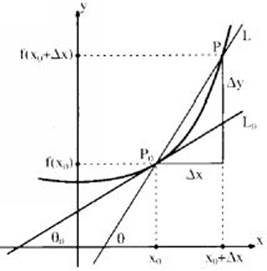
a. A straight line tangent to the graph of function , if it exists, is the line obtained as the limit of straight lines when point tends to (see illustration).

Equivalently, the tangent straight line to the graph at , is the limit of straight line when tends to zero.

b. is the slope of the straight line tangent to the graph of the function at , and there holds when is the angle between the tangent line and the positive direction of the -axis.

c. The tangent equation is .

4.3 Linear Approximation

a. Function , defined at a specific neighborhood of point is differentiable at if, and only if, there exists a constant and there exists function , for which holds such that

b. If is differentiable, then for a small enough , we write . That is, the graph of function can be approximated to a straight line in a small enough neighborhood of .

c. If function is differentiable at , then it is continuous at this point.

d. Not any function continuous at is differentiable at .

Example: is continuous at but not differentiable at .

4.4 Derivative Rules

Let be derivable functions, and a constant.

Therefore:

f. Chain Rule: Derivative Composite Functions

If is function derivable at , and is function derivable at , then the composite function is derivable at , and there holds the equality:

In other words, the derivative of composite function equals to the derivative of multiplied by the derivative of its inner function .

g. Derivative Inverse Function

If is invertible function in the neighborhood of , differentiable at , and, then is inverse function, , is differentiable at , and there holds

h. Derivative functions in the form of when :

Using the logarithm function , we differentiate:

Using another way: and deriving.

i. Deriving a Function Presented in its Parametric Form:

Let be a function given in the parametric form of , (see II.3), when is invertible in the given domain, that is , and therefore, . Then, from chain rule, there follows:

4.5 Derivatives of Elementary Functions


		9.			1.
		10.			2.
		11.			3.
		12.			4.
		13.			5.
		14.			6.
		15.			7.
		16.			8.

4.6 One-Sided Derivatives

a. If function is defined in a right-handed neighborhood of , and there exists limit , it is called the right-hand derivative of at , and is denoted by .

b. The left-handed derivative of at is

c. Example: The one-sided derivatives of are

d. The function is differentiable at if, and only if, its one-sided derivatives at exist are equal.

e. If the derivative at exists, then .

f. Function is differentiable in close interval , if it is differentiable at and its one-sided derivatives , exist.

4.7 High-Order Derivatives

a. Let be a function derivable at interval . If we derivative it at all points of the interval, we'll have a new function , which, too, is defined in all interval . The function is the first derivative of in interval .

If function , also, is derivable in interval , we will denote its derivative as . is defined on all interval , and is called the second derivative of . Similarly, we define the third derivative, forth derivative, and so on.

In general, if function can be derivated times, in interval , then, the last function in the set of derivatives is denoted by or by , and is called the -th derivative of .

Another denotation of -th derivative is that of Leibniz: .

b. Leibniz formula

Let and be functions differentiable times at . Then:

when .

c. Examples:

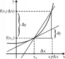
4.8 Differentials

1. The entity is called the differential of at point . As opposed to variable, which does not depend on any other entity, the variable depends on and .

Another basic essential difference between and is that while , usually, . The illustration shows the geometric description of each of these entities, and the way the entity is related to entity. These two entities tend to unite as decreases.

2. If , then .

b. Higher-Order Differentials

is a second-order differential.

is an -th order differential.

4.9 Differential Calculus Basic Theorems

1. Fermat’s Theorem

Let be a function defined on open interval and differentiable at inner point . If attains a maximum or a minimum value at , then .

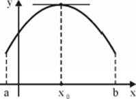
2. The Geometric Meaning of Fermat's Theorem

If attains a maximum or a minimum value at , and if, in the neighborhood of , its graph has a “hill,” then, the straight line tangent to at this point have to parallel to the -axis. That is, the derivative at should be zero.

b. Rolle's Theorem

Let be a function defined at close interval , and there holds the following:

1. is continuous at close interval .

2. is differentiable at open interval .

3. .

Then, there is a , such that .

Geometrically, Rolle's theorem means that if a continuous and differentiable function at a close interval has equal values at the extreme points of the interval, then there exists at least one point within the interval where the straight line tangent to the graph is parallel to the -axis. But sometimes, there is more than one such point.

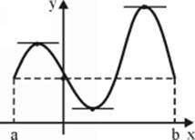
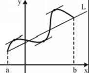
c. Lagrange's Mean-Value Theorem

1. If is a function continuous at close interval and differentiable at open interval , then there is at least one point c, such that

2. Geometrically, the theorem means that if is a function continuous at close interval and differentiable at open interval , then there exists a point on the graph where the straight line tangent to the graph in it is parallel to the straight line passing through the extreme points of the graph. The illustration shows the graph of a function with three such points.

3. Another form of Lagrange's theorem: if is a function differentiable at interval , then, for all , such that , there exists a real number , , such that

d. Cauchy's Mean-Value Theorem

1. Let and be two functions continuous at close interval and differentiable at open interval , and, in addition, for all . Then, there is at least one point c, , such that

2. If and are functions continuous and differentiable in the neighborhood of , and, for all in that neighborhood, then, for every , (small enough) such that is in the given neighborhood, there exists a real number , , such that

e. Darboux's Mean-Value Theorem

1. If function is differentiable at close interval , then for every between and there exists an such that . In other words, if is differentiable at the close interval , then, the image of is an interval.

2. If function is differentiable at close interval , then its derivative is not necessarily continuous and therefore is not differentiable.

If is not continuous at , then it is a second-type discontinuity.

Example: The derivative of 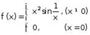is function 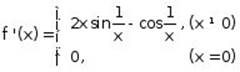, which is not continuous at , since the limit does not exist.

4.10 L'Hopital's Rules

a. Let and be functions differentiable in the neighborhood of , except, possibly, at . Suppose that:

1. There exists the limit

or .

2. for all in the neighborhood of .

3. There exists the limit .

Then, there also exists the limit , and there holds that .

b. If functions and are differentiable in infinite interval (a,∞), and

1. The limits exist

2. for all

3. The limit exists.

Then, the limit also exists, and there holds .

4.11 Taylor's Formula

a. If function is differentiable times in the neighborhood of , and is a point in this neighborhood, then there exists a point , between and , such that

when is Lagrange remainder.

If, we substitute in Taylor's formula, we obtain Maclaurin formula:

b. Peano Remainder Formula

c. Cauchy Remainder Formula

d. Examples:

4. ,

4.12 Investigations of Function

a. Intervals of Increase and Decrease of a Function:

1. Differentiable Function is constant in interval if, and only if, for all .

2. is not decreasing in interval if, and only if, .

3. is not increasing in interval if, and only if, .

4. is increasing in interval if, and only if, for all .

5. is decreasing in interval if, and only if, , for all .

Note: Propositions 4 and 5 are true one-way only. That is, if is differentiable and monotone increasing in interval , then, it doesn’t necessarily follow that for all points of . For example, is increasing in yet .

b. Local Maximum and Minimum Values:

1. has a local minimum value at if there exists a definite neighborhood of where there holds for all in this neighborhood.

2. has a local maximum value at if there exists a definite neighborhood of where there holds for all in this neighborhood.

Point , which is a local minimum or maximum, is called a local extreme point or local extremum of .

3. A necessary condition for the existence of local extremum: If function is differentiable in then neighborhood of extreme point , then .

4. is called a critical point of if . Critical points and points in which is not differentiable are called suspected extremum points.

c. Sufficient Condition of Extremum

1. Let be a function defined in the neighborhood of . The sign of is said to change from negative to positive at , if there exists a neighborhood , such that for all in the interval , , and, for all in the interval , . The same way we determine when the sign of changes from negative to positive at . maintains its sign in point , if there exists a neighborhood where for all of, or for all in this neighborhood.

2. First Derivative Test

Let be a suspected extremum point of function , if is continuous in , and is differentiable in the neighborhood of , except, possibly, in , then follows:

a) If the sign of changes from negative to positive in , then is a local minimum of .

b) If the sign of changes from positive to negative in , then is a local maximum of .

c) If maintains its sign at , then is not a local extremum of .

3. Second Derivative Test

If is a critical point of and is twice differentiable, then follows:

a) If then is a local minimum of .

b) If then is a local maximum of .

c) If , then we cannot conclude on from this method, and we should examine it using the previous method or other ways.

d. Absolute Maximum and Minimum in Domain

1. Point is an absolute maximum of in domain if, for all , there holds .

2. Point is called absolute minimum of in domain if, for all , there holds .

e. Concavity and Points of Inflection

1. Function is concave down on interval , if, for all and for all , there holds

2. Function is concave up on interval , if, for all and for all , there holds

3. If function is differentiable on , and there exists an neighborhood of where the graph of the function is under the tangent line to the graph at that point, that is, there exists an such that, for all which holds there holds , Then is concave down on .

4. Function is concave up on , if there exists a neighborhood of where the graph of is above the tangent line to the graph at that point.

5. Function is concave down on open interval , if it is concave down on any point of the interval. Similarly, we define concavity up on interval .

6. Sufficient Condition of Concavity

Let be a function twice differentiable on interval , then:

a) If, for all in interval , , then is concave up in interval .

b) If, for all in interval , , then is concave down in interval .

f. Points of Inflection

Point is the point of inflection of function , if is continuous at and there exists a neighborhood such that the concavity directions of the function in intervals , are opposite. That is, if is concave down in interval and concave up in interval , or vise versa.

g. Asymptotes

1. The straight line is a vertical asymptote of function , which is defined in a right-handed or left-handed neighborhood of point , except, possibly, , if, at least one of the limits , equals to or .

2. The geometric meaning of the existence of vertical asymptote is that the graph of , near point , gets steep and very close to the straight line , but doesn't contact it.

3. The straight line is an oblique asymptote of at , when .