CHEMICAL BIOLOGY
Membranes, Fluidity of
Boris Dzikovski and Jack H. Freed, Department of Chemistry and Chemical Biology, Advanced Center for ESR Technology (ACERT), Cornell University, Ithaca, New York
doi: 10.1002/9780470048672.wecb313
In the popular fluid mosaic model for biomembranes, membrane proteins and other membrane-embedded molecules are in a two-dimensional fluid formed by the phospholipids. Such a fluid state allows free motion of constituents within the membrane bilayer and is extremely important for membrane function. The term ''membrane fluidity'' is a general concept, which refers to the ease of motion for molecules in the highly anisotropic membrane environment. We give a brief description of physical parameters associated with membrane fluidity, such as rotational and translational diffusion rates, order parameters etc., and review physical methods used for their determination. We also show limitations of the fluid mosaic model and discuss recent developments in membrane science that pertain to fluidity, such as evidence for compartmentalization of the biomembrane by the cell cytoskeleton.
Introduction
In 1972, Singer and Nicolson (1) suggested the so-called fluid mosaic model of the biological membrane (Fig. 1) (2). This useful hypothesis explained many phenomena that occur in model and biological membranes. According to this model, membrane proteins and other membrane-embedded compounds are suspended in a two-dimensional (2-D) fluid formed by phospholipids. The phospholipids are assumed to be in a liquid state, so they are capable of rapid diffusion within their layer and are in constant motion. This fluid state of membrane lipids is critical for membrane function. It allows, for example, free diffusion and equal distribution of new cell-synthesized lipids and proteins, lateral diffusion of proteins and other molecules in signaling events and other membrane reactions, membrane fusion (i.e., fusion of vesicles with organelles), separation of membranes during cell division, and so on.
Generally speaking, two principal mechanisms operate in the biology of membrane processes, such as membrane transport and permeation. One involves a network of active sites and operates by metabolic energy, and it is referred to as active; another is directed by passive diffusion, and it is called passive. This passive mechanism is determined by various aspects of lipid dynamics and lipid-protein interactions, and it can be described in quantitative terms of chemical and phase equilibrium and molecular physics. However, in the highly anisotropic membrane environment, some aspects must be generalized and redefined compared with the simple isotropic case. One term, which received a new interpretation in the context of membrane science, is “fluidity.” Membrane fluidity, which describes the ease of movement for molecules in the membrane environment, is a general concept that lacks a precise definition. It is much broader than the strict physical definition of fluidity as the reciprocal of viscosity in the case of isotropic liquids. In general, “membrane fluidity” implies various anisotropic motions, which contribute to the mobility of components of a membrane. It includes lateral diffusion of molecules in the plane of the membrane, flexibility of acyl chains, “flip-flop” diffusion of molecules from one monolayer to the other, and so on. The most important parameters to quantify the notion of membrane fluidity are translational and rotational diffusion constants, order parameters (or tensors), packing, and permeability. In general, greater membrane fluidity is associated with higher diffusion rates, high permeability, lower ordering, and looser packing. The relation between the parameters, however, is purely empirical, and in most cases speculative. Many membranes have large diffusion constants and large order parameters and vice versa.
The lipid membrane, as a whole, shows a unique combination of fluidity and rigidity. In terms of the solubility and the diffusion of small nonpolar molecules, the membrane behaves very much like an oil drop. In contrast, the translational diffusion constants of lipids and proteins in membranes are characteristic of media with the viscosity over two orders of magnitude greater than that of oil, such as hexadecane. Also, in most cases the membrane represents an impermeable barrier for ions and other hydrophilic compounds.
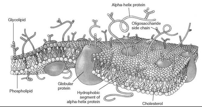
Figure 1. Singer-Nicolson model of fluid membrane. (From Reference 2.)
Physical Parameters Associated with Membrane Fluidity
Diffusion constants
Diffusion is the random movement of a particle because of an exchange of thermal energy with its environment. Membrane lipids and proteins participate in highly anisotropic translational and rotational diffusion motion. Translational diffusion in the plane of the membrane is described by the mean square lateral displacement after a time ∆t: ![]() Lipid lateral diffusion coefficients in fluid phase bilayers are typically in the range DT ~ 10-8 to 10-7 cm2/s (3).
Lipid lateral diffusion coefficients in fluid phase bilayers are typically in the range DT ~ 10-8 to 10-7 cm2/s (3).
Rotational diffusion is characterized by the mean square angular deviation during the time interval ∆t: ![]() Highly anisotropic motion, which is typical for lipid molecules in the membrane, is usually described by two rotational diffusion coefficients DRll and DR⊥, which correspond to diffusion about the long diffusion axis and perpendicular to it, respectively. The diffusion coefficients are related to corresponding rotational correlation times measured by nuclear magnetic resonance (NMR), electron spin resonance (ESR), fluorescent depolarization, and so on, as:
Highly anisotropic motion, which is typical for lipid molecules in the membrane, is usually described by two rotational diffusion coefficients DRll and DR⊥, which correspond to diffusion about the long diffusion axis and perpendicular to it, respectively. The diffusion coefficients are related to corresponding rotational correlation times measured by nuclear magnetic resonance (NMR), electron spin resonance (ESR), fluorescent depolarization, and so on, as:
![]()
Forfluid phase bilayers, the typical rotational diffusion coefficients are of the order of ![]() and
and ![]()
![]() (3). This example can help in visualizing lipid motion in the membrane: for an area per lipid of 60 A2 with DRll and DT of 4-108 s-1 and 1-10-8 cm2/s, correspondingly, one can observe that a lipid molecule travels a distance of approximately the width of its headgroup on the membrane surface, while rotating once around its long axis, which is directed along its hydrocarbon chain. A value of DT of 10-8 cm2/sec, typically measured for lipids in biomembranes, corresponds to a net distance traversed of about 2 μm in 1 second.
(3). This example can help in visualizing lipid motion in the membrane: for an area per lipid of 60 A2 with DRll and DT of 4-108 s-1 and 1-10-8 cm2/s, correspondingly, one can observe that a lipid molecule travels a distance of approximately the width of its headgroup on the membrane surface, while rotating once around its long axis, which is directed along its hydrocarbon chain. A value of DT of 10-8 cm2/sec, typically measured for lipids in biomembranes, corresponds to a net distance traversed of about 2 μm in 1 second.
Flip-flop diffusion
Lipid molecules, in principle, can exchange between the two monolayers of the bilayer. For polar lipids, it is an extremely slow process with characteristic times of hours or even days (4). For membrane proteins, no appreciable flip-flop mobility has yet been observed, which is in good accord with the fact that inner and outer leaflets of natural membranes are usually asymmetric with respect to their protein and lipid composition. On the other hand, cholesterol has a relatively high rate of spontaneous flipping between two membrane leaflets (t1/2 ~ 1s) (5).
Order parameters
The membrane lipid layer is a lamellar phase with the preferred orientation of the lipid molecules perpendicular to the membrane plane. By definition, if θ is the angle of the long molecular axis with respect to the bilayer normal, then the order parameter S, which is a measure of the orientation distribution, is given as the average of P2(cos θ), the second Legendre polynomial: ![]() (6). One can see that S varies between -1/2 and 1. These limiting cases have the following meaning: when S = 1, all molecules are exactly perpendicular to the membrane plane. When S = -1/2, θ = 90°, and all molecules have their long axis parallel to the membrane surface. The case of S = 0 usually corresponds to a random distribution of molecular axes relative to the membrane normal. In energy terms, the rotation of the molecular long axis in the liquid crystal is restricted within an orienting potential that is simply approximated as: U(θ) = λ∙cos2 θ, where λ is the strength of the potential. The ordering of the lipid chain relative to the bilayer normal can then be expressed (7) as:
(6). One can see that S varies between -1/2 and 1. These limiting cases have the following meaning: when S = 1, all molecules are exactly perpendicular to the membrane plane. When S = -1/2, θ = 90°, and all molecules have their long axis parallel to the membrane surface. The case of S = 0 usually corresponds to a random distribution of molecular axes relative to the membrane normal. In energy terms, the rotation of the molecular long axis in the liquid crystal is restricted within an orienting potential that is simply approximated as: U(θ) = λ∙cos2 θ, where λ is the strength of the potential. The ordering of the lipid chain relative to the bilayer normal can then be expressed (7) as:
Permeability
The passive permeability of lipid membranes is another fluidity related parameter. In general, two mechanisms of membrane permeability can operate in the membrane (8). For many nonpolar molecules, the predominant permeation pathway is solubility-diffusion, which is a combination of partitioning and diffusion across the bilayer, both of which depend on lipid fluidity. In a few cases, such as permeation of positively charged ions through thin bilayers, an alternative pathway prevails (9, 10). It is permeation through transient pores produced in the bilayer by thermal fluctuations. This mechanism, in general, correlates with membrane fluidity. However, for model membranes undergoing the main phase transition, permeation caused by this mechanism exhibits a clear maximum near the phase transition point (11).
Phase State and Membrane Fluidity
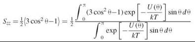
A remarkable property of lipid bilayers is their structural phase transitions (thermotropic polymorphism). For example, fully hydrated pure diacyl-phosphatidyl cholines exibit one fluid phase, La and three crystalline phases: Pβ’, L β’, and Lc (12). Because of the high degree of disorder caused by defects, the Pβ’ and Lβ’ phases usually are called gel phases. The Pβ’ phase is sometimes called a “ripple phase,” because the surface of the bilayer is rippled (13) and presents a wave-like appearance in electron micrographs (Fig. 2). Depending on the nature of the lipid and the presence of additional components (cholesterol etc.), the Pβ’ phase may be present or absent in the phase diagram, and a tilted gel Lβ’ could be replaced by the Lβ phase, which has similar physical properties but no tilt of the hydrocarbon chains.
In the gel phase, lipid chains are usually well aligned with little rotation around the C-C bonds that are predominantly in the trans position. The lipid chains are tightly packed, the chain ordering is high, the bilayer thickness is maximal, and the surface area per lipid headgroup is relatively small. Lipids in the gel phase in most cases can be handled as solids. For example, aligned thick multibilayers in the gel phase can be sliced in thin pieces in an arbitrary direction so that each piece retains macroscopic alignment (14). The physiological importance of gel-like phases is limited.
At the “main transition” temperature, Tm, the gel phase undergoes a transition to the La (liquid crystal) phase. At the transition point, the surface area increases (15), and the bilayer thickness and chain order decrease (16). In the fluid phase, hydrocarbon chains tend to contain more gauche isomers (17). At this transition, the DSC (differential scanning calorimetry) shows a sharp peak in the heat capacity that occurs over a narrow temperature range. The transition between Lβ’ and Pp/ phases also can be detected by DSC and is called the pretransition (18). The transition between Lc and Lβ’phases is in most cases hard to observe because of typical supercooling of the Lβ phase. Depending on the membrane composition, hydration, and temperature, several 2-D and three-dimensional nonlamellar lipid phases are possible, including the well-studied hexagonal (HI and HII) and cubic phases (19).
Natural biomembranes contain a complex mixture of various phospholipids with cholesterol and sphingomyelins. In general, they exist in the fluid phase. Maintaining membrane fluidity seems to be extremely important for the survival of the cell and the whole organism. It is well known for model membranes that a decrease in the chain length or the introduction of unsaturation into the hydrocarbon chain causes a decrease in the main transition temperature. Consistent with this observation, microorganisms, plants, and animals (poikilotherms or hibernating mammals) are acclimated to low temperatures by altering their membrane lipid composition, increasing the degree of lipid unsaturation, or decreasing the average chain length (20-23).
In an attempt to relate natural and model membranes, many lipid mixtures have been examined experimentally. It has been shown that additional components broaden the main phase transition, with a wider temperature range of coexisting gel and liquid phases (24). Another important feature of lipid mixtures is the formation of nonideal solutions with nonzero enthalpy and/or entropy of mixing. It often makes the components completely or partially immiscible in one or both phases and manifests itself in complex phase diagrams (25).
Cholesterol, which is an important constituent of cell membranes, plays an important role in maintaining membrane fluidity. It effectively inhibits the transition to the gel phase (26, 27). Even though some plasma membranes, such as nerve myelin membranes, contain a high concentration of lipids that form gel phase bilayers, the presence of cholesterol keeps these membranes in a fluid phase. However, interaction with the rigid cholesterol ring affects hydrocarbon chains of lipids in the liquid crystal phase (La) and leads to formation of a new phase, the liquid ordered (Lo) phase (27). The phase is well characterized by a variety of physical methods and does not exist in pure lipids or their mixtures. In the liquid ordered phase, the long axis rotation and lateral diffusion rates are similar to the La phase, but the acyl chains are predominantly in an all-trans conformation and, hence, the order parameters are similar to the Lβ phase (see Table 1). Recently, the cholesterol-rich Lo phase has been strongly associated with microdomains in live cells—the so-called “lipid rafts.”
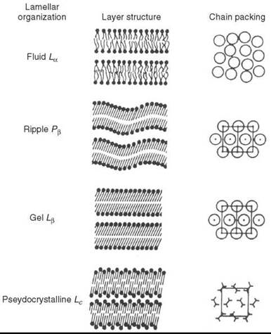
Figure 2. Organization of the lamellar bilayer phases of DPPC in the fluid (La), ripple (Pβ), gel (Lβ’) and pseudo-crystalline (Lc) states. A top view of the packing of the hydrocarbon chains is shown in the last column. (From Reference 12.)
Table 1. Translational diffusion coefficients of lipids and order parameters in some membrane phases
|
Phase |
DT |
S* |
|
Liquid-crystalline (La) |
10-8 cm2/s |
0-0.2 |
|
Gel (Lβ) |
10-11 cm2/s |
0.2-0.9 |
|
Gel (Pβ’) |
Similar to Lβ, but the bilayer is rippled |
|
|
Gel (Lβ’) |
The same as Lβ, but the chains are tilted 32° |
|
|
Liquid-ordered (Lo) |
10-8 cm2/s |
0.2-0.9 |
* Measured by NMR
Physical Methods for Measuring Fluidity Parameters
In the membrane environment, a wide range of motions has been observed and studied by a variety of physical methods. The characteristic times of the motions span 20 orders of magnitude, from about 10-14 s for molecular vibration to days for transbilayer flip-flops. Figure 3 shows characteristic frequencies (reciprocal of characteristic times) of different kinds of molecular motions in the membrane in comparison to frequency ranges in which various spectroscopic techniques are sensitive to molecular motion (28).
A spectroscopic technique that probes membrane fluidity can either directly measure mobility and order parameters for membrane constituents (NMR) or use probes (ESR, fluorescence). Some fluorescent and ESR probes are shown in Fig. 4. The connection between the rotational correlation time of a membrane embedded probe and the membrane fluidity can be illustrated using the example of a simple isotropic liquid, in which fluidity is merely a reciprocal viscosity n and the rotational correlation time τc for a molecule with a hydrodynamic volume V is given by the well-known Debye-Stokes-Einstein relation: τc = ηV/kT, where k is the Boltzmann constant and T is the absolute temperature; the rotational diffusion coefficient (DR) is given by DR = 1/6Tc.
In the highly anisotropic membrane environment, one can expect several different correlation times that correspond to the anisotropic membrane environment and/or the nonspherical molecular probe as well as variations that exist along the membrane normal within the bilayer. Furthermore, the molecular motion is often limited by constraints imposed by the ordered surroundings of the probe. Properly designed spectroscopic experiments can, in many cases, extract both mobility and order parameters and can give a comprehensive picture of membrane fluidity.
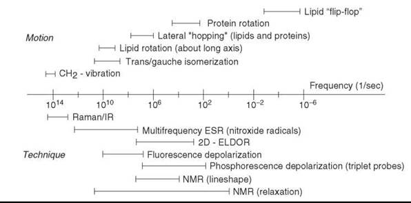
Figure 3. The characteristic frequencies of molecular motions of membrane proteins and lipids compared with the frequency ranges in which various spectroscopic techniques are sensitive to molecular motion. (Modified from Reference 28.)
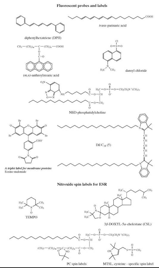
Figure 4. Probes for fluorescence studies and ESR spectroscopy.
Fluorescent experiments for measuring molecular mobility and ordering
Absorption of a photon instantaneously brings the probe molecule to the first excited singlet state S1. Usually it takes ~10—8 seconds to return to the ground state. It can occur via collision with neighbors and loss of the energy as heat or through the emission of a photon (fluorescence). The fluorescence lifetime (TF) is the characteristic time for the population of excited molecules to return to the ground state after a flash of excitation light.
The fluorescence depolarization technique for mobility and ordering is based on the fact that the probability of absorption and emission is directional. Light polarized along a certain axis will preferably excite molecules oriented with their transition dipole moment in the same direction. The probability varies with cos2 θ, where 0 is the angle between the transition dipole moment and the electric field vector of the light. Emission of a photon obeys the same cos2 θ (28) rule. That means that a molecule oriented with its transition dipole moment along the Z-axis will be likely to emit a photon with the same polarization. In the depolarization technique, polarizers are used to quantify the intensity of the parallel (Ill) and perpendicular (I⊥) components to the original direction of polarization.
The values of Ill and I⊥ are used to obtain the anisotropy ![]() If no molecular motion occurs between the time of absorption and time of emission (TC » TF), then molecules tend to emit in the direction of original polarization, Ill > I⊥ and r has a maximal value equal 0.4. In the opposite limit (TC » TF, and isotropic rotation) the molecules will emit in a random direction, Ill = I⊥ and r = 0. In the intermediate range, for
If no molecular motion occurs between the time of absorption and time of emission (TC » TF), then molecules tend to emit in the direction of original polarization, Ill > I⊥ and r has a maximal value equal 0.4. In the opposite limit (TC » TF, and isotropic rotation) the molecules will emit in a random direction, Ill = I⊥ and r = 0. In the intermediate range, for ![]() the value of r is sensitive to molecular motions.
the value of r is sensitive to molecular motions.
An important advantage of the depolarization technique is that it allows one to measure the molecular ordering, as well as the motional parameters. For this purpose, it is necessary to detect the time dependence of the anisotropy. In the presence of ordering constraints, the r value does not decay to zero, but to some limiting value r∞: r = ![]() The rate of decay defines a rotational correlation time, and ris a direct measure of the order parameter through the following relation: s2 = r∞/r0 (29). The fluorescence depolarization method works well as long as fluorescence lifetimes, which are typically ~10—8 s, are not too different from the rotation relaxation times to be measured. When the rotational correlation time is slower than about 10—6 s, however, the method fails because the fluorescent emission decays before any detectable rotation can occur. For studying rotational diffusion of membrane proteins, it is almost always the case that correlation times are in the microsecond time range or longer, because membranes are at least 100 times more viscous than water. Several phosphorescent probes (e.g., derivatives of eosin) were developed to measure such slow rotation correlation times. In such molecules, after initial excitation, transition into the lowest triplet state T1 (intersystem crossing) effectively competes with S1-S0 transition. Because the T1-S0transition is spin forbidden, the lifetime of the lowest triplet state (typically 10—3 s) is much longer than that of the S1 (typically 10—8-10—9 s).
The rate of decay defines a rotational correlation time, and ris a direct measure of the order parameter through the following relation: s2 = r∞/r0 (29). The fluorescence depolarization method works well as long as fluorescence lifetimes, which are typically ~10—8 s, are not too different from the rotation relaxation times to be measured. When the rotational correlation time is slower than about 10—6 s, however, the method fails because the fluorescent emission decays before any detectable rotation can occur. For studying rotational diffusion of membrane proteins, it is almost always the case that correlation times are in the microsecond time range or longer, because membranes are at least 100 times more viscous than water. Several phosphorescent probes (e.g., derivatives of eosin) were developed to measure such slow rotation correlation times. In such molecules, after initial excitation, transition into the lowest triplet state T1 (intersystem crossing) effectively competes with S1-S0 transition. Because the T1-S0transition is spin forbidden, the lifetime of the lowest triplet state (typically 10—3 s) is much longer than that of the S1 (typically 10—8-10—9 s).
Solid state NMR
Solid state NMR is characterized by relatively broad lines. It can be described as magnetic resonance on molecules frozen in solids or with very slow rotational correlation times. It is appropriate not only for solids, but also for viscous solvents, lipids in membranes, or large macromolecules in solution. High resolution (solution) NMR deals with relatively small molecules with molecular weight less than about 50,000 Da in aqueous solution. The rotation of such molecules is so fast on the NMR time scale that it effectively averages out all orientational anisotropy yielding an isotropic spin Hamiltonian including the Zeeman term and the J-J coupling with another spin S; ![]() Here, I and S are spin operators for two nuclear spins, B0 is the external magnetic field strength, yN is the magnetogyric ratio for the studied nucleus; σ is the chemical shielding constant, which is directly related to the chemical shift δ; J is the spin-spin coupling constant for spins I and S. For no or very slow rotational reorientation the spin Hamiltonian requires a tensorial expression:
Here, I and S are spin operators for two nuclear spins, B0 is the external magnetic field strength, yN is the magnetogyric ratio for the studied nucleus; σ is the chemical shielding constant, which is directly related to the chemical shift δ; J is the spin-spin coupling constant for spins I and S. For no or very slow rotational reorientation the spin Hamiltonian requires a tensorial expression: ![]() where
where

are chemical shielding and spin-spin coupling tensors.
Tensor values should also be assigned to quadrupole splittings (see below).
The tensor σ is usually symmetrical, and in the appropriate molecular frame it is represented in a diagonal form:
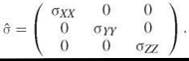
The components σXX, σYY, and σZZ give chemical shifts along main molecular axis in X-, Y-, and Z- direction, respectively. When the molecule is oriented along the main axis, for example the Z-direction, the chemical shift is just azz. Other orientations give intermediate values. In the limiting case of absence of molecular motion (rigid limit) and a statistical distribution of molecular orientations, for example polycrystalline or glass, the spectrum shows a superposition of spectra for all orientations.
Routinely, NMR study of membrane structure and dynamics uses 31P or 2H nuclei (30-32).
Phosphorus 31 has spin I = 1/2. The chemical shift tensor is substantially anisotropic. For static, statistically disordered molecules, the spectrum is a superposition of spectra that correspond to different orientations. If the molecule undergoes fast rotation about one axis, then the motion averages the components perpendicular to that axis. In the case of fast isotropic rotation (limiting case of high resolution NMR), a single sharp line is observed in the spectrum (Fig. 5). For example, the rotation of the vesicle depends on its size and the viscosity of the environment. The smaller the vesicle, the faster is the rotation. Very fast isotropic tumbling of the vesicle gives a single isotropic peak. For large vesicles, however, the spectrum corresponds to anisotropic rotation of the lipid molecule itself about the main axis.
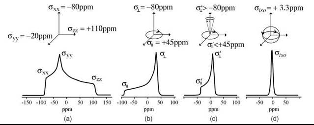
Figure 5. 31P-NMR spectra of phospholipids with different modes of molecular motion. a: rigid limit; b: fast axial rotation about X-axis averages Y- and Z-components of the chemical shift tensor. In the spectrum one can observe two principal values of ![]() and σll = σ⊥; c: a typical case of fluid membrane. Along with fast X-axial rotation molecular motion also partially averages σll and σ⊥. In the spectrum one observes effective values σ'| < σ|| and σ'⊥ < σ⊥: Isotropic case (high resolution NMR):
and σll = σ⊥; c: a typical case of fluid membrane. Along with fast X-axial rotation molecular motion also partially averages σll and σ⊥. In the spectrum one observes effective values σ'| < σ|| and σ'⊥ < σ⊥: Isotropic case (high resolution NMR): ![]()
Diffusion along the membrane surface affects the averaging of tensor components, especially if the surface is curved. Lipids can form other aggregates than bilayer membranes. For instance, a common form is the inverse hexagonal phase (HII-phase). It consists of cylindrical lipid tubes with the lipid hydrocarbon chains on the outside and directed radially and the water phase in the center. Diffusion of lipids leads to a different type of anisotropic averaging of the tensor components than in the case of large vesicles. Figure 6 (33) shows 31P-NMR spectra from lipids in the bilayer membrane, the HII phase and the isotropic case. If a lipid system undergoes the La—HII transition, then the 31P-NMR lineshape abruptly changes at the transition temperature as shown in Fig. 6.
Use of 2H-NMR for membrane studies is based on the fact that deuterium nuclei, with spin I = 1, have an electric quadrupole moment. It originates from the asymmetrical charge distribution in the nucleus. In the presence of an external field gradient, which is almost always the case for (deuterium) atoms in molecules, the different orientations of the nuclear spin experience different interaction energies with the quadrupolar field of the environment.
Figure 6. 31 P-NMR spectra in various membrane phases. (From Reference 33.)
For a system with spin 1 and the absence of any quadrupo- lar interaction, one has three spin energy levels in the external magnetic field for mI = —1, 0, +1. They have the same energy splitting between adjacent levels, which yield only one resonance line. Through the quadrupole interaction, the energy levels are no longer equidistant, and one observes two resonance lines. If the quadrupolar splitting is much less than the Zeeman splitting is, then the approximate expression for a fixed orientation of the molecule is (34):
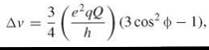
where eQ is the quadrupole moment, eq is the magnitude of the principal component of the gradient of the electric field, and ф is the angle between the direction of that component and the external magnetic field. The two resonance lines are split by a frequency of ∆v. For the special case of ф = 54.7° (magic angle), ∆v = 0 and no quadrupole splitting occurs. A superposition of all orientation gives a sum of two broad spectra that are symmetrical about the central resonant frequency, which is a lineshape similar to a Pake doublet for two interacting protons in a single water molecule.
For fast rotation (the case of high resolution NMR), the quadrupolar splitting is averaged out yielding a single resonance line. For intermediate cases, the splitting and the line shape of the quadrupolar NMR signal is indicative of the rotational correlation time and/or ordering effects (Fig. 7) (30).
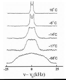
Figure 7. 2H-NMR spectra at 23.3 MHz of 1-[16,16,16-2H] palmitol,2-palmitoleoyl-PC at different temperatures. (From Reference 30.)
ESR spectroscopy
Although theoretically NMR can obtain both molecular dynamics and ordering, a close look at the literature shows that in membranes, NMR is used mostly for extracting order parameters. Much information on rotational mobility of membrane constituents is traditionally obtained using another magnetic resonance technique, ESR. ESR is extremely useful in the study of membrane fluidity, because of its unique time scale, which spans almost all motional range in membranes.
For studies of membrane fluidity, lipids or membrane proteins are usually spin-labeled with cyclic nitroxide radicals. The theoretical analysis of the spin Hamiltonian of ESR is analogous to that for NMR, although the interaction terms are much larger. The position of ESR lines for nitroxides is determined by the g-factor and the hyperfine splitting, which roughly correspond to the chemical shift and J-J coupling in NMR, and the sensitivity of ESR spectroscopy to molecular motion emerges from the dependence of these parameters on the orientation of the nitroxide moiety in the magnetic field.
The ESR-Hamiltonian is given as ![]() where S and I are spin operators for electrons and nuclei; g and A—g- and A-tensors of the radical,
where S and I are spin operators for electrons and nuclei; g and A—g- and A-tensors of the radical, ![]() is the Bohr magneton;
is the Bohr magneton; ![]() is the magnetogyric ratio for the electron, ge, the g-factor for free electron, is 2.002319, and B0 is the applied magnetic field strength.
is the magnetogyric ratio for the electron, ge, the g-factor for free electron, is 2.002319, and B0 is the applied magnetic field strength.
Similar to fluorescence depolarization and NMR, two limiting cases exist in which the molecular motion becomes too slow or too fast to further effect the ESR lineshape (Fig. 8) (35). At the fast motion limit, one can observe a narrow triplet centered around the average g value (gxx + gyy + gzz)/3 with a distance between lines of aiS0 = (Axx + Ayy + Azz)/3, where gii and Aii are principal values of the g-tensor and the hyperfine splitting tensor A, respectively. At the slow motion limit, which is also referred to as the rigid limit, the spectrum (shown in Fig. 8) is a simple superposition of spectra for all possible spatial orientations of the nitroxide with no evidence of any motional effects. Between these limits, the analysis of the ESR lineshape and spectral simulations, which are based on the Stochastic Liouville Equation, provide ample information on lipid/protein dynamics and ordering in the membrane (36).
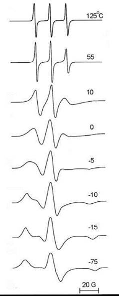
Figure 8. ESR spectra of TEMPO nitroxide radical in glycerol at different temperatures. (From Reference 35.)
For the most common ESR frequency of 9 GHz, the limits are approximately from 10-7 < τc < 10-11 seconds. However, using a range of ESR frequencies and pulse and continuous wave (CW) ESR techniques (such as ELDOR or saturation transfer ESR) expands the range from 10-4 to ~ 10-12 seconds, which covers virtually all modes of molecular motion in the membrane that can be associated with membrane fluidity (37). In the past, to study the range of 10-7-10-4 seconds, an empirical technique known as saturation transfer ESR was used. It is based on detection of an out-of-phase ESR signal with large modulation amplitude (typically 5G) of the external magnetic field (38). The most direct way to observe the “saturation transfer” is ELDOR or electron-electron double resonance, when two different microwave frequencies are applied to the sample. One is called the “pump” frequency and used to modify the populations by saturating certain portions of the ESR spectrum. Another one (the “probe” frequency) is used to observe the effect of the “pump” frequency on other parts of the spectrum. The response to an intense (saturating) microwave field is affected by diffusion of saturation (“saturation transfer”) between different portions of the resonance spectrum. In the case of nitroxide labels, this diffusion is dominated by rotational modulation of the anisotropic magnetic interactions. The method is most sensitive when the rotational correlation time is comparable with or greater than the spin lattice relaxation time, which for nitroxides near the rigid limit is ~10-5seconds. In the CW mode, usually the intensity of the ESR signal at the “probe” frequency is recorded as a function of the “pump” frequency. A huge improvement has been achieved by using the Pulsed Two-Dimensional Fourier Transform technique, which is known as 2-D ELDOR. This experiment very efficiently provides all combinations of pump and probe frequencies in a single 2-D experiment, and in addition it dramatically improves the spectral resolution, which enables accurate assessment of mobility and ordering parameters. As observed in Fig. 9 (39), 2-D ELDOR spectra show dramatic changes as membrane properties are varied.
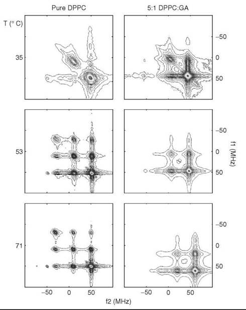
Figure 9. 2D-ELDOR spectra for DPPC membranes containing spin-label 16PC (cf. Fig. 4) with and without gramicidin A at different temperatures. (From Reference 39)
Lateral Diffusion in Membranes
As we will see later, studying lateral diffusion in biomembranes gives important insights into their structure and function. Methods for measuring diffusion coefficients for lipids in membranes can be classified into two distinct categories. (40) In the first category, which corresponds to short-range diffusion measurements, D is obtained from determination of frequencies of bimolecular collisions within the membrane, through fluorescence, ESR, and so on. In the second category, which corresponds to long-range diffusion measurements, D is usually determined from the time required to fill a defined region of the membrane.
Short-range lateral diffusion
ESR is very useful in the study of dynamic properties of membrane components because of its high sensitivity and favorable time scale. Early ESR studies of short-range lateral diffusion in membranes were based on Heisenberg exchange (HE) effects of nitroxide spin-label linewidth. The HE contribution to the ESR linewidth is given for 14N nitroxides by ![]() where d is the encounter distance for two spin-bearing molecules, D is the microscopic self-diffusion coefficient, NA is the Avogadro number, and C is the molar concentration of spins (41). The factor f can be deduced from the assumed model of intermolecular potential energy for the interaction between two spins. For a simple, hard-sphere potential f ≡ 1. The technique based on direct determination of changes in the ESR linewidth because of HE (42) was later improved by using ELDOR and/or saturation recovery. These techniques are based on the effects of the HE on saturation transfer between hyperfine lines of the spin labels, and they allow one to detect substantially lower HE rates. Additional improvement of this technique based on use of 14N-15N spin-label pairs gave ~20-fold in the sensitivity and allowed experiments on cells (43).
where d is the encounter distance for two spin-bearing molecules, D is the microscopic self-diffusion coefficient, NA is the Avogadro number, and C is the molar concentration of spins (41). The factor f can be deduced from the assumed model of intermolecular potential energy for the interaction between two spins. For a simple, hard-sphere potential f ≡ 1. The technique based on direct determination of changes in the ESR linewidth because of HE (42) was later improved by using ELDOR and/or saturation recovery. These techniques are based on the effects of the HE on saturation transfer between hyperfine lines of the spin labels, and they allow one to detect substantially lower HE rates. Additional improvement of this technique based on use of 14N-15N spin-label pairs gave ~20-fold in the sensitivity and allowed experiments on cells (43).
For the measurements of short-range diffusion, the collision rate can also be obtained by optical spectroscopy from fluorescence quenching. In the isotropic case of diffusion-controlled dynamic quenching, the change in fluorescence intensity obeys the equation:
![]()
where Ф0 and Ф are the quantum yield in the absence and presence of quencher, respectively; (Q) is the concentration of quencher, and KSV is referred as the Stern-Volmer constant, which is related to the diffusion coefficient by the Smoluchowski equation. However, the isotropic and three-dimensional theory of fluorescence quenching does not apply in the membrane, and a Stern-Volmer modified treatment has been developed for this case (44).
Long-range diffusion measurements
For studying long-range diffusion, many studies have been conducted using the technique of fluorescence recovery after photo- bleaching (FRAP) (45). The translational diffusion coefficients that can be measured using this technique range from about 10-7 to 10-12 cm2/s. For a small area of the membrane, that contains fluorescent-labeled molecules of interest, the initial level of fluorescence is determined. Then, a flash of intense laser beam is applied irreversibly to bleach a substantial (100% in the ideal case) fraction of fluorophores in this area, so it appears black after the flash. The intensity of the laser light for the bleaching is typically ~103 times greater than the light used to monitor the fluorescence. For the bleached area, the fluorescence intensity is recorded as a function of time. The brightness will gradually increase as fluorescent molecules diffuse into this area. Two parameters are determined from a FRAP experiment (Fig. 10):
1. The lateral mobility, which gives the diffusion coefficient directly and is determined by the slope of the fluorescent recovery curve. The steeper the curve, the more mobile the molecules.
2. The percent recovery, which is determined as (Y/X) x 100 = % recovery. It gives the mobile fraction of the probe. If the radius of the illuminated area is small compared with the diffusion area (cell, vesicle, etc.) and the molecules are free to diffuse, then the percent recovery must be 100%. On the other hand, if the fluorescence fails to recover to the same intensity observed before the bleaching pulse, then it indicates that a fraction of fluorophores exist, which are immobile on the time scale of the experiment (DT < 10-12cm2/s).
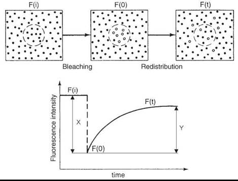
Figure 10. FRAP experiment. (From Reference 28.)
In recent years, FRAP for diffusion measurements in membranes has been superseded by fluorescence correlation spectroscopy (FCS). FCS is very similar to FRAP in both theoretical and experimental approaches to the observation of diffusion. The difference between these two closely related techniques is that FRAP measures relaxation from an initial nonequilibrium state after photobleaching, whereas FCS detects stochastic fluctuations that occur even in a system remaining in equilibrium (46).
ESR techniques for studying long-range diffusion usually observe the spreading of a small region of concentrated spins over time. For diffusion rates typical of a membrane environment, the most appropriate method is dynamic imaging of diffusion by ESR (DID-ESR) (47), which has been used to measure 10-5 > DT > 10 10 cm2/s. The measurement of the diffusion coefficient, D, by DID-ESR involves two stages. After preparing the sample with an inhomogeneous distribution of spin probes along a given direction, the investigator uses the ESR imaging method to obtain the (one-dimensional) concentration profiles at several different times. Spatial resolution results from a magnetic field gradient, because spin probes at each spatial point experience a different resonance frequency. With time, the inhomogeneous distribution will evolve toward a homogeneous distribution via translational diffusion. The second stage is to fit the time-dependent concentration profiles to the diffusion equation to obtain D. The ESR spectrum recorded in the presence of a magnetic field gradient B’ (G/cm) is a convolution of the usual ESR spectra (gradient-off spectrum), I0(%), with the concentration of spins C(x, t), which initially varies along the direction x: ![]()
Here, ξ ≡ (B-B0) measures the spectral position as the deviation of the magnetic field B from the field B0 at the center of the spectrum, which corresponds to the position x = 0, because the field gradient B' maps x onto %, as given by ξ = B'x. The determination of C(ξ, t) from the two spectra Ig(ξ, t) and I0(ξ) is a straightforward calculation through Fourier transformation. Fitting the C(ξ, t) profile to the diffusion equation gives the diffusion rate.
Pulse field gradient (PFG) NMR spectroscopy is now generally regarded as the method of choice for measuring the translational diffusion coefficients of molecules of virtually any type under many conditions (48). 1H, 2H, 19F, and 31P variants of this method have been used successfully to study lateral diffusion of cholesterol, phospholipids, and water in model membranes (49, 50). This technique introduces two identical gradient pulses of the external magnetic field into the standard spin-echo NMR rf pulse sequence, one is between the π/2 and π pulses and another is after the π pulse. If spins do not undergo any translational diffusion, then the effect of the two applied gradient pulses cancels out and after the rf π-pulse the echo refocuses to the same value as in the absence of the gradient. However, the diffusion movement of spins between the gradient pulses causes additional dephasing, which cannot be refocused by the π-pulse and manifests itself in a decrease in the resulting echo intensity. The degree of dephasing is proportional to the displacement of spins in the direction of the gradient and, hence, the translational diffusion rate.
In the last decade, motion of lipid and protein single molecules in biomembranes was studied extensively by either single-particle tracking or by ultra-sensitive single-molecule fluorescent microscopy or fluorescence correlation spectroscopy. In single-particle tracking, a particle of typical diameter of 30-50 nm is attached to the lipid or protein molecule as a label. Colloidal gold and fluorescent particles have been used as labels. The particle motion is then followed by computer-enhanced video microscopy. Single-molecule fluorescence measurements are based on the repetitive excitation of a single fluorophore, which generates repeated cycles of absorption and fluorescence and count rates of up to tens of thousands of counts per second. The fluorescence is detected by single-photon counting modules.
Lipids diffuse freely in fluid model membranes. FRAP measurements show full recovery and diffusion coefficients on the order of magnitude of 10-8 cm2/sec. Free diffusion with a similar rate is often observed for lipids in the biomembrane. However, many cell membrane proteins show lower diffusion rates and incomplete recovery after photobleaching. For membrane proteins, dramatically different behavior in model and biological membranes is a common case. In model membranes, membrane proteins also diffuse freely and their diffusion coefficients are often similar to the diffusion coefficients of lipids. On the contrary, in biomembranes, the diffusion of proteins is 2-3 orders of magnitude slower and the fluorescence recovery is often incomplete. This observation points to limitations of the fluid mosaic model as will be discussed below.
Fluidity Versus Mosaicity—New Concepts in Membrane Science
The Singer-Nicolson model of the membrane played a very important role in understanding membrane structure and function. However, many properties of biomembranes are not consistent with this model. In recent years, a growing consensus points at more complex membrane structure, which can be characterized as “dynamically structured fluid mosaic.” Compared with the original fluid mosaic model, the emphasis has shifted from fluidity to mosaicity. Experimental observations have led to the “membrane microdomain” concept that describes compartmentalization/organization of membrane components into stable or transient domains.
One observation, which is inconsistent with the simple fluid mosaic model, is the reduced diffusion coefficients of membrane molecules in the plasma membrane compared to model membranes and biomembranes deprived of their cytoskeleton (blebs). Another observation is the oligomerization-induced slowing of diffusion (51). It manifests itself in much greater effect of diffusant size on the translational diffusion rate than predicted by the theory of Saffman-Delbruck based on the Singer-Nicolson model (52). If a transmembrane protein is approximated as a rigid cylinder of radius r and height h, floating in a two-dimensional liquid of viscosity n with matching thickness (h) surrounded by an aqueous medium of viscosity η1, then the theory gives the following expression for its translational diffusion coefficient DT:
![]()
where γ is the Euler constant (≈ 0.577216). This formula predicts very weak dependence of translational diffusion on the size of diffusant. For example, for a 10-fold increase in the protein radius, from 5 to 50 A, the theory predicts for a 50-A thick bilayer a decrease in the diffusion rate by a factor of 1.57. Another factor of 10-increase in the radius, which corresponds to a 75-fold increase in the aggregation number, slows the diffusion rate by a factor of 2.6. Although this insensitivity looks somehow counterintuitive, the Saffman-Delbruck formula gives good results for proteins incorporated into model membranes.
On the contrary, for the plasma membrane, the effect of oligomerization on the diffusion rate is much stronger than predicted by the formula. For example, for linked couples of green fluorescent protein-E-cadherin oligomerization with an aggregation number between 2 and 10 slows down the diffusion up to 40 times (53). Also, spectacular single-particle tracking experiments carried out by Kusumi et al. (51) showed that in natural biomembranes, the diffusion does not follow usual Brownian patterns but consists of a series of random Brownian walks within confined areas (compartments) followed by longer-distance hops between compartment. (see trajectory in Fig 11) (54). The compartment size varies depending on the cell nature but is relatively insensitive to the diffusant, which shows the same size for transmembrane proteins and phospholipids. For example, in the case of normal rat kidney epithelial cells, the average compartment size is 230 nm with an average residency time within the compartment ~11 ns (51).
The hop-diffusion pattern cannot be found in liposomes or membrane blebs. In these membranes, the membrane molecules show simple Brownian diffusion with a single diffusion coefficient (55).
Because the assumption of simple Brownian diffusion breaks down, the diffusion in biomembranes cannot be described by a single diffusion coefficient. For instance, FRAP experiments in the plasma membrane showed that the observed translational diffusion rates depend on the size of the initial photobleached spot, which is also inconsistent with a simple Singer-Nicolson model.
Accumulating evidence clearly points at involvement of the cell cytoskeleton in the compartmentalization of the membrane, in particular, the fine cytoskeleton filaments formed by actin in most eukaryotic cells or spectrin in mammalian red blood cells. However, single-particle tracking experiments show the same patterns of hop-diffusion for lipid molecules located in the extracellular leaflet of the plasma membrane. How can the membrane skeleton, which is located only on the cytoplasmic surface of the membrane, suppress the motion of lipids on the extracellular side?
To reconcile this apparent contradiction the membrane skeleton fence and anchored transmembrane picket model was proposed (54). According to this model, transmembrane proteins anchored to and lined up along the membrane skeleton (fence) effectively act as a row of posts for the fence against the free diffusion of lipids (Fig. 11). This model is consistent with the observation that the hop rate of transmembrane proteins increases after the partial removal of the cytoplasmic domain of transmembrane proteins, but it is not affected by the removal of the major fraction of the extracellular domains of transmembrane proteins or extracellular matrix. Within the compartment borders, membrane molecules undergo simple Brownian diffusion. In a sense, the Singer-Nicolson model is adequate for dimensions of about 10 x 10 nm, the special scale of the original cartoon depicted by the authors in 1972. However, beyond such distances simple extensions of the fluid mosaic model fail and a substantial paradigm shift is required from a two-dimensional continuum fluid to the compartmentalized fluid.
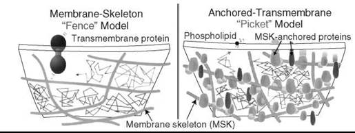
Figure 11. Membrane skeleton fence and anchored transmembrane picket model. (From Reference 51.)
Acknowledgment
This work was supported by grants from NIH NCRR and NIH NIBIB.
References
1. Singer SJ, Nicolson GL. The fluid mosaic model of the structure of cell membranes. Science 1972; 175:720-731.
2. Bretscher MS. The molecules of the cell membrane. Scientific Am. 1985; 253:100-108.
3. Marsh D. CRC Handbook of Lipid Bilayers. 1990. CRC Press, Boca Raton, FL.
4. Homan R, Pownall HJ. Transbilayer diffusion of phospholipids: dependence on headgroup structure and acyl chain length. Biochim. Biophys. Acta 1988; 938:155-166.
5. Lange Y, Dolde J, Steck TL. The rate of transmembrane movement of cholesterol in the human erythrocyte. J. Biol. Chem. 1981; 256:5321-5323.
6. Tsvetkov V. Acta physicochimica USSR. 1942; 16:132.
7. Chandrasekhar S. Liquid Crystals. 1977. Cambridge University Press, Cambridge, UK.
8. Volkov AG, Paula S, Deamer DW. Two mechanisms of permeation of small neutral molecules and hydrated ions across phspholipid bilayers. Bioelectrochem. Bioenerget. 1997; 42:153-160.
9. Langner M, Hui SW. Dithionite penetration through phospholipid bilayers as a measure of defects in lipid molecular packing. Chem. Phys. Lipids 1993; 65:23-30.
10. Hamilton RT, Kaler EW. Alkali metal ion transport through thin bilayers. J. Phys. Chem. 1990; 94:2560-2566.
11. Papahadjopoulos D, Jacobsen D, Nir K, Isac T. Phase transitions in phospholipid vesicles. Fluorecsence polarization and permeability measurements concerning the effect of temperature and cholesterol. Biochim. Biophys. Acta 1973; 311:330-348.
12. Jain MK. Introduction to Biological Membranes. 1988. Wiley, New York.
13. Janiak, MJ, Small DM, Shipley GG. Nature of the thermal pretransition of synthetic phospholipids: dimyristolyl- and dipalmitoyllecithin. Biochemistry 1976; 15:4575-4580.
14. Dzikovski BG, Earle KA, Pachtchenko SV, Freed JH. High-field ESR on aligned membranes. A simple method to record spectra from different membrane orientations in the magnetic field. J. Magnet. Reson. 2006; 179:273-277.
15. Seddon JM, Templer RH. Polymorphism of lipid-water systems. In: Handbook of Biological Physics. Lipowsky R, Sackmann E, eds. 1995. Elsevier Science, Amsterdam, The Netherlands. pp. 97-160.
16. Heimburg T. Mechanical aspects of membrane thermodynamics. Estimation of mechanical properties of lipid membranes close to the chain melting transition from calorimetry. Biochim. Biophys. Acta 1998; 1415:147-162.
17. Mendelson R, Davies MA, Brauner JW, Schuster HF, Dluhy RA. Quantitative determination of conformational disorder in the acyl chains of phospholipid bilayers by infrared spectroscopy. Biochemistry 1989; 28:8934-8939.
18. Cunningham BA, Brown AD, Wolfe DH, Williams WP, Brain A. Ripple phase formation in phosphatidylcholine: Effect of acyl chain relative length, position, and unsaturation. Phys. Rev. E 1998; 58:3662-3672.
19. Gruner SM. Nonlamellar lipid phases. In: The Structure of Biological Membranes. Yeagle PL, ed. 1992. CRC Press, Boca Raton, FL. pp. 211-250.
20. Goldman SS. Cold resistance of the brain during hybernation. III. Evidence of lipid adaptation. Am. J. Physiol. 1975; 228:834-838.
21. Combos Z, Wada H, Murata N. Unsaturation of fatty acids in membrane lipids enhances tolerance of Cyanobacterium synechocystis PCC6803 to low-temperature photoinhibition. Proc. Natl. Acad. Sci. U.S.A. 1992; 89:9959-9963.
22. Pruitt NL. Membrane lipid composition and overwintering strategy in thermally acclimed crayfish. Am. J. Physiol. 1988; 254:R870-876.
23. McElhaney RN. The relationshhip between membrane fluidity and phase state and the ability of bacteria and mycoplasmas to grow and survive at various temperatures. Biomembranes 1984; 12:249-276.
24. Mabrey S, Sturtevant JM. High-sensitivity differential scanning calorimetry in the study of biomembranes and related model systems. In: Methods in Membrane Biology. Korn EDE, ed. 1978. Plenium Press, New York. pp. 237-274.
25. van Dijk PWM, Kaper AJ, Oonk HAJ, De Gier J. Miscibility properties of binary phosphatidylcholine mixtures. A calorimetric study. Biochim. Biophys. Acta 1977; 470:58.
26. Lewis RNAH, McElhaney RN. The mesomorphic phase behaviour of lipid bilayers. In: The Structure of Biological Membranes. Yeagle PE, ed. 1991. CRC Press, Boca Raton, FL. pp. 73-155.
27. Ipsen JH, Karlstrom G, Mouritsen OG, Wennerstrom H, Zuk- ermann MJ. Phase equilibria in phosphatidylcholine-cholesterol system. Biochim. Biophys. Acta 1987; 905:162-172.
28. Gennis RB. Biomembranes. Molecular structure and function. 1989, Springer Verlag, New York.
29. Heyn MP. Determination of lipid order parameters and rotational correlation times from fluorescence depolarization experiments. FEBS Lett. 1979; 108:359-364.
30. Davis JH. The description of membrane lipid conformation, order and dynamics by 2H-NMR. Biochim. Biophys. Acta 1983; 737:117-171.
31. Seelig J. 31P Nuclear magnetic resonance and the head group structure of phospholipids in membranes. Biochim. Biophys. Acta 1978; 515:105-140.
32. Iuga A, Ader C, Groger G, Brunner E. Applications of solid-state 31P NMR spectroscopy. Ann. Reports NMR Spectros. 2006; 60:145-189.
33. Aloia RC, ed. Membrane Fluidity in Biology, Volume 1. 1983. Academic Press, New York. Chapter 2.
34. Abragam, A., The Principles of Nuclear Magnetism. 1983. Oxford University Press, New York.
35. Kuznetsov AN. The Spin Probe Method [in Russian]. 1976. Nauka, Moscow.
36. Schneider DJ, Freed JH. Calculating slow motional magnetic resonannce spectra: a user’s guide. In: Biological Magnetic Resonance. Berliner LJ, Reuben J, eds. 1989. Plenum Publishing Corporation, New York. pp. 1-76.
37. Freed JH. New technologies in electron spin resonance. Ann. Rev. Phys. Chem. 2000; 51:655-689.
38. Marsh D, Horvath L, Pali T, Livshits VA. Saturation transfer spectroscopy of biological membranes. In: Biomedical ESR. Eaton GRESS, Berliner LJ, eds. 2004. Kluwer Academic/Plenum Publishing, New York. pp. 309-368.
39. Costa-Filho AJ, Crepeau R, Borbat P, Mingtao G, Freed JH. Lipid-gramicidin interactions: dynamic structure of the boundary lipid by 2D-ELDOR. Biophys. J. 2003; 84:3364-3378.
40. Tocanne J-F, Dupou-Cezanne L, Lopez A. Lateral diffusion of lipids in model and natural membranes. Progr. Lipid Res. 1994; 33:203-237.
41. Shin Y-K, Ewert U, Budil DE, Freed JH. Microscopic versus macroscopic diffusion in model membranes by electron spin resonance spectral-spatial imaging. Biophys. J. 1991;59:950-957.
42. Trauble H, Sackmann E. Studies of the crystalline-liquid crystalline phase transition of lipid model membranes. III. Structure of a steroid-lecitin system below and above the lipid-phase transition. J. Am. Chem. Soc. 1972; 94:4499-4510.
43. Lai CS, Wirt MD, Yin JJ, Froncisz W, Feix JB, Kunicki TJ, Hyde JS. Lateral diffusion of lipid probes in the surface membrane of human platelets. An electron-electron double resonance (ELDOR) study. Biophys. J. 1986; 50:503-506.
44. Owen CS. Two dimensional diffusion theory: Cylindrical diffusion model applied to fluorescence quenching. J. Chem. Phys. 1975; 62:3204-3207.
45. Vaz WLC, Derzko ZI, Jacobson K. Photobleaching measurements of the lateral diffusion of lipids and proteins in artificial phospholipid bilayer membranes. Cell Surface Rev. 1982; 8:83-135.
46. Webb WW. Fluorescence correlation spectroscopy: inception, biophysical experimentations, and prospectus. Applied Optics 2001; 40:3969-3983.
47. Freed JH. Field Gradient ESR and molecular diffusion in model membranes. Ann. Rev. Biophys. Biomolec. Struct. 1994; 23:1-25.
48. Price WS. Pulsed-field gradient nuclear magnetic resonance as a tool for studying translational diffusion: part 1. Basic theory. Conc. Magnet. Reson. 1997; 9:299-336.
49. Filippov A, Oradd G, Lindblom G. Lipid lateral diffusion in ordered and disordered phases in raft mixtures. Biophys. J. 2004; 86:891-896.
50. Lindblom G, Oradd G, Filippov A. Lipid lateral diffusion in bilayers with phosphatidylcholine, sphingomyelin and cholesterol. An NMR study of dynamics and lateral phase separation. Chem. Phys. Lipids 2006; 141:179-184.
51. Kusumi A, et al. Paradigm shift of the plasma membrane concept from the two-dimensional continuum fluid to the partitioned fluid: high-speed single-molecule tracking of membrane molecules. Ann. Rev. Biophys. Biomolec. Struct. 2005; 34:351-378.
52. Saffman PG, Delbrilck M. Brownian motion in biological membranes. Proc. Natl. Acad. Sci. U.S.A. 1975; 72:3111-3113.
53. Iino R, Koyama I, Kusumi A. Single molecule imaging of green fluorescent proteins in living cells: E-cadherin forms oligomers on the free cell surface. Biophys. J. 2001; 80:2667-2677.
54. Ritchie K, Iino R, Fujiwara T, Murase K, Kusumi A. The fence and picket structure of the plasma membrane of live cells as revealed by single molecule techniques. Molec. Membr. Biol. 2003; 20:13-18.
55. Fujiwara T, Ritchie K, Murakoshi H, Jacobson K, Kusumi A. Phospholipids undergo hop diffusion in compartmentalized cell membrane. J. Cell Biol. 2002; 157:1071-1081.
Further Reading
Davis JH. The description of membrane lipid conformation, order and dynamics by 2H-NMR. Biochim. Biophys. Acta 1983; 73:117-171.
Freed JH. New technologies in electron spin resonance. Ann. Rev. Phys. Chem. 2000; 51:655-689.
Marsh D. CRC Handbook of Lipid Bilayers. 1990. CRC Press, Boca Raton, FL.
Slichter CP. Principles of Magnetic Resonanse. 3rd edition. 1990. Springer Verlag, New York.
Tocanne J-F., Dupou-Cezanne L, Lopez A. Lateral diffusion of lipids in model and natural membranes. Progress Lipid Res. 1994; 33:203-237.
Webb WW. Fluorescence correlation spectroscopy: inception, biophysical experimentations and prospectus. Appl. Optics 2001; 40:3969-3983.
Yeagle P, ed. The Structure of Biological Membranes. 1992. CRC Press, Boca Raton, FL.