Liquid-State Physical Chemistry: Fundamentals, Modeling, and Applications (2013)

9.2. Molecular Dynamics

The core of MD simulations is the solution of Newton's equations of motion (see Chapter 2), as applied to molecules, given the set-up of the previous paragraph. Denoting²⁾ for particle i with mass m_i at any time t the force by f_i, the momentum by p_i and the coordinates by r_i, these equations read

(9.1)

For forces that can be derived from a (time-independent) potential Φ (r), Newton's laws lead to a conservation of energy

(9.2)

Correctly solving these equations leads to the trajectories of the various molecules. Since in this approach, representing the micro-canonical (or NVE) ensemble, the number of molecules N, total volume V and the total energy Eare constant, the conjugate variables show fluctuations. In this representation the temperature is a fluctuating average of the kinetic energy which can be derived at any moment from the equipartition theorem, that is, via

(9.3)

where ⟨···⟩ denotes the time average. The time average is taken to yield the same answer as the ensemble average. Although the total energy E is in principle conserved, in practice the unavoidable discretization of the time steps needed to solve the equations of motion will cause integrations errors and the total energy E will not be exactly conserved. Therefore, T may drift even after equilibrium has been reached.

In order to simulate the canonical (or NVT) ensemble, the temperature must be controlled, and to do this the system is coupled to a temperature bath or thermostat. This is in essence a model of the “outside world”, constructed in such a way that the energy exchange is comparable to that of a system coupled to a large environment but still yielding fast answers. Introducing in the same way a barostat to regulate pressure, the pressure (or NPT) ensemble results. Finally, employing a similar strategy for particles, the grand-canonical (or μVT) ensemble can be simulated. For nonequilibrium simulations the thermostat (and other “stats”) should represent the external driving forces which determine that the system responds to changes continuously. Finally, if one wants to make use of the fluctuations to calculate higher-order thermodynamic properties, the nature of the “stats” is also important. For example, the optimal choice of a thermostat will differ for different purposes, for example, to reach equilibrium or to correctly estimate fluctuations.

For practical calculations, Eq. (9.1) is replaced by an equation with finite time steps of length Δt. The algorithm for integrating the MD equations should satisfy a few basic requirements. The first of these is that on a microscopic level, time reversal symmetry (as required by Newton's equations) should be conserved. The second requirement, normally denoted as the symplectic requirement, is that upon integration the equation of motion the area and volume in phase space should be conserved. If not obeyed, the equilibrium distributions are also not conserved and may show spurious time dependences. The third requirement is that preferably for each time step only one evaluation of the force f_i is needed, because computationally this is by far the most expensive step. This is due partially to the large number of pairs, in principle N(N − 1)/2, for which a calculation is required, and partially due to the (possibly) complex form of the potentials used.

There are various ways to satisfy these requirements, but the most commonly used algorithm is due to Verlet [7]. Using a Taylor expansion we write for r_i(t ± Δt) around t

(9.4)

so that adding the forward and reverse forms leads to

(9.5)

If Eq. (9.5) is truncated after the Δt² term, the resulting expression is called Verlet's algorithm and in essence it estimates the accelerations as

(9.6)

So, for updating the coordinates the velocities are not explicitly required. Provided that or, using the force and its second derivative, , the effect of the Δt⁴ term is small as compared to the Δt²term. Typically, this requires Δt to be of the order of 10⁻¹⁵ s, which imposes a serious practical restraint on the total time that the system can be followed. The constancy of the energy E can be used as a check of whether Δt is small enough, but this requires the velocities to be known. The latter we easily obtain from the Verlet algorithm as

(9.7)

An estimate accurate [8] to is obtained by adding [f_i(t − Δt) − f_i(t + Δt)]Δt/12m_i to Eq. (9.7). Using the Verlet algorithm the system propagates along a trajectory in space.

To start a simulation one needs an initial set of coordinates that can be obtained in various ways. A logical first choice would be to be minimize the potential energy, that is, a T = 0 K calculation. The second option is to use the final configuration of a simulation with nearby conditions. A third option is to use a lattice on which the N particles are located at t = 0. When using Verlet's algorithm, one clearly needs a configuration at t = −Δt. This configuration may be constructed by giving molecules a Maxwell–Boltzmann distribution for some temperature T at t = 0, that is,

(9.8)

From this distribution we pick at random³⁾ values for p_i/m_i for i = 1, 2, … , N and use

(9.9)

which represents the distance a molecule would have traveled with a fixed velocity from t = −Δt to t = 0.

After starting the calculation we compute the trajectory from one state at t = t to the next at t = t + Δt. The kinetic temperature, as defined by Eq. (9.3), normally rises significantly after any sort of arbitrary initial configuration. This is due to the fact the particle has to find its way to a lower state of potential energy under the influence of the intermolecular interactions. After a sufficient number of time steps, the average temperature is reached. In case of the NVT ensemble, one way to control the temperature is by scaling the velocities with a factor x, typically according to

(9.10)

and thereafter calculate r_i(t + Δt) from r_i(t) and for i = 1,2, … , N leading to a change of temperature from T to T′ = x²T. More sophisticated thermostats are the Andersen and Nosé–Hoover thermostats. In the Andersen thermostat, the coupling to a heat bath is represented by stochastic impulsive forces that act by now and then on randomly selected particles. The strength of the coupling should be chosen before the simulation starts. It can be shown that this thermostat indeed generates a canonical ensemble, but it is not very useful for nonequilibrium simulations as the sudden impulse change leads to nonrealistic fluctuations. The Nosé–Hoover thermostat employs an extended Lagrange function that can be used in nonequilibrium simulations, but only in the case the system has only one constant of the motion. In nonequilibrium simulations this is the case, since in that case the total momentum is not conserved (for the system we consider) because of the externally applied force. In an equilibrium simulation this condition is fulfilled if the center of mass of the system is fixed. This restrictive condition of only one constant of the motion may be alleviated by using a sequence of Nosé–Hoover thermostats. For details, we refer to the literature⁴⁾.

Generally it will take many time steps, perhaps 10³ to 10⁴, before a situation is reached that represents the equilibrium fluctuations of the system. Logging all data provides the possibility of plotting most quantities of interest as a function of time. Often – and in particular when the time step is small enough – the configuration changes little per time step, and one uses only data at every nth step, where n may be 10 or more. Calculating the property for a number of consecutive time segments we may estimate the statistical variation. This process is comparable to an experimental repetition to obtain an estimate of the experimental errors. Advanced methods exist to eliminate time correlation⁴⁾, although systematic errors cannot be assessed so easily. For example, the use of a finite size N-particle system automatically confirms that correlations for a length larger than the cell are suppressed, even when the energy expression implies such a correlation. Moreover, there is the question of how efficiently a phase space can be sampled. For sufficiently short-ranged potentials, correlation and sampling are not serious problems, but for systems where long-range correlations play an important role – for example, in crystallization or for systems with relatively deep, metastable potential wells, perhaps larger than 5 kT or 10 kT, at a density near the close-packed value – they are important.

For any property f the time average over the n steps is constructed according to

(9.11)

where f_i is the value for f at step i. Taking the potential energy as an example we have

(9.12)

For the temperature we obtain . Using the fluctuations in energy (see Section 5.1), the heat capacity C_V results from

(9.13)

Another way to calculate C_V is to use the temperature coefficient of the average internal energy E_ave, that is, potential plus kinetic energy, as obtained from simulations at various temperatures. This is usually a more satisfactory method. The pressure can be calculated from the virial theorem expression (see Chapter 3) reading

(9.14)

with ∇_j the gradient operator for molecule j. Last but not least, if we use for f_i the number of particles n(r) located at a distance between r and r + Δr from a reference particle, and taking subsequently each particle as reference, the average value ⟨n(r)⟩ is directly related to the pair correlation function according to

(9.15)

provided that Δr is small enough so that the change in g(r) in this range is small.

Although the intention is to eliminate the surfaces, the sensitivity of the averages on the periodic boundary conditions depends inversely on the number of particles N, while the computational effort is of for simulations with a short-range potential using a cut-off. For long-range interactions, using clever summation techniques, the efforts scales as . However, for a larger N value it takes fewer time steps n to reach a given accuracy [see Eq. (9.11)and (9.12)]. If all particles contribute directly to the average of interest, the number of data points varies as Nn, so that the cost may be more nearly proportional to N, subject to computer memory limitations. The method outlined here may be applied not only to spherical molecules such as Ar, but also to systems of more complex molecules. One can then either use the rigid molecule approximation and describe the system by “generalized coordinates” such as orientational coordinates and their associated momenta, or use flexible molecules with appropriate potentials for bond stretching, bond bending, and dihedral torsion. For details, we refer to the literature.

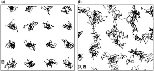
To illustrate this method, snapshots of the pioneering simulations by Alder and Wainwright [9] are shown in Figure 9.2. Here, Figure 9.2a shows the projected trajectories of a hard-sphere system in the solid state, and demonstrates that the atoms, on average, are largely fixed at their equilibrium position. Figure 9.2b shows the trajectories in the liquid state for those atoms which move throughout the complete volume of the cell.

Figure 9.2 Trajectories for 3000 collisions in (a) the solid state and (b) the liquid state of a 32-particle hard-sphere system at V/V₀ = 1.525 projected on a plane.

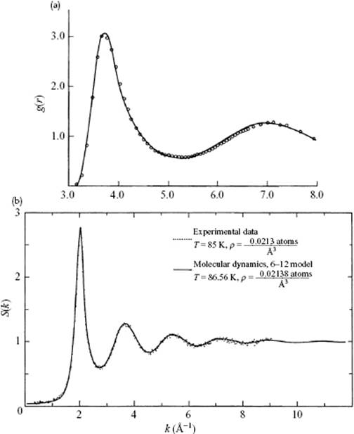
As a final example, we compare in Figure 9.3 the pair-correlation function of Ar, as calculated by the MD method using the LJ potential with experimental results (note the very good agreement). Nowadays, much more elaborate simulations can be carried out, for which a number of software packages are currently available.

Figure 9.3 (a) The pair correlation function for liquid Ar at T = 86.56 K and ρ = 0.02138 Å⁻³, near its triple point. The solid line represents the results of a MD simulation for a 6–12 potential (σ = 3.405 Å, ε/k = 119.8 K) chosen to fit the thermodynamic data for Ar. The MD result is indistinguishable from MC results, including three-body interactions. The circles represent the result of Fourier inversion of the S(s) curve in panel (b); (b) Neutron diffraction data S(s) for liquid Ar compared with model calculations with data as given for panel (a).

Problem 9.1

Verify Eq. (9.7) and its extension.

Problem 9.2

What are the advantages and disadvantages of more sophisticated updating schemes for r_i?