Liquid-State Physical Chemistry: Fundamentals, Modeling, and Applications (2013)
11. Mixing Liquids: Molecular Solutions
11.8. Empirical Improvements*
In this section we indicate briefly some empirical improvements that can be made on the regular solution model, largely based on an expansion of the excess Gibbs function. Theoretical improvements deal with a better description for the local configuration than being based on random mixing with consequences for entropy and energy, and we discuss these in the next section.
The excess Gibbs energy as used in the regular solution model can be systematically but largely empirically extended. As a first approximation in the regular solution model, we wrote ![]() , where wm is a (temperature-dependent) parameter (we omit the subscript m from now on). Corrections on this expression may be modeled as a power law in x1 and x2. Hence, we can write the Redlich–Kister expansion [8]
, where wm is a (temperature-dependent) parameter (we omit the subscript m from now on). Corrections on this expression may be modeled as a power law in x1 and x2. Hence, we can write the Redlich–Kister expansion [8]
(11.115) ![]()
The inclusion of these terms generates systematic improvements in the description.
When A = B = C = ··· = 0, GE = 0, RTlnγ1 = RTlnγ2 = 0 and γ1 = γ2 = 1. Accordingly, we regain the ideal solution.
When B = C = ··· = 0, GE = Ax1x2 and ![]() and
and ![]() . Obviously, these results represent the regular solution and the expressions are symmetric in nature. For infinite dilution one obtains
. Obviously, these results represent the regular solution and the expressions are symmetric in nature. For infinite dilution one obtains ![]() .
.
When C = ··· = 0, GE/x1x2 = A + B (x1 − x2), implying a deviation from the regular solution model. Equivalently, since x1 + x2 = 1, we may write GE/x1x2 = A (x1 + x2) + B (x1 − x2) or defining A21 = A + B and A12 = A − B,
(11.116) ![]()
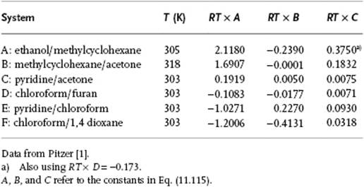
a result known as the Margules equation. Obviously, this approach can be extended although, according to Guggenheim [9], an expansion further than third order is hardly ever required in view of the experimental accuracy. In Figure 11.7 and Table 11.5 some examples are presented of GE functions, which shows that this approach is flexible and can describe rather different type of behaviors, that is, continuously increasing GE, continuously decreasing GE, and a GE showing a maximum or minimum.
Figure 11.7 Excess Gibbs energies for the systems of Table 11.5.
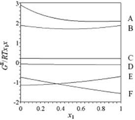
Table 11.5 Excess Gibbs function parameters for various solutions.
One may also expand the reciprocal x1x2/GE in the mole fractions to obtain the van Laar expansion [10]
(11.117) ![]()
Equivalently, we may write, since (x1 + x2) = 1,
(11.118) ![]()
Defining ![]() and
and ![]() , we obtain
, we obtain
(11.119) ![]()
The expressions for the activity coefficients, known as the van Laar equations, are
(11.120) ![]()
In this case for x1 = 0, ![]() and for x2 = 0,
and for x2 = 0, ![]() .
.
Some algebraic manipulation, meanwhile, identifying ![]() and
and ![]() , where Vα is the partial volume of component α and C is a constant, shows that Eq. (11.119) is equivalent to an expansion of GE in the volume fraction ϕ1 = V1x1/(V1x1 + V2x2) = V1x1/Vm, where Vm ≡ V1x1 + V2x2 is the molar volume of the mixture, that is,
, where Vα is the partial volume of component α and C is a constant, shows that Eq. (11.119) is equivalent to an expansion of GE in the volume fraction ϕ1 = V1x1/(V1x1 + V2x2) = V1x1/Vm, where Vm ≡ V1x1 + V2x2 is the molar volume of the mixture, that is, ![]() . This relation fits data well for many binary systems of normal liquids. In the van Laar version the constant C was originally given in terms of the a- and b-parameters of the vdW equation, that is
. This relation fits data well for many binary systems of normal liquids. In the van Laar version the constant C was originally given in terms of the a- and b-parameters of the vdW equation, that is
(11.121) ![]()
To be preferred is the expression, rationalized by Scatchard [11],
(11.122) ![]()
where ΔUα = ΔvapHα − RT is the molar energy of vaporization, and the solubility parameter δα = (ΔUα/Vα)1/2 is used. The latter expression is also given by the approximate statistical mechanical calculation in Section 11.6. Using ![]() and
and ![]() as parameters, the ratio
as parameters, the ratio ![]() corresponds reasonably well to V1/V2, for example, for the mixture benzene and iso-octane [12] at 45 °C
corresponds reasonably well to V1/V2, for example, for the mixture benzene and iso-octane [12] at 45 °C ![]() , while experimentally V1/V2 = 0.536.
, while experimentally V1/V2 = 0.536.
Although these expressions show a relatively large flexibility in fitting the experimental data, their theoretical basis is flimsy and the equations are difficult to extend to multicomponent systems. Finally, the temperature dependence of the parameters involved is not explicitly included. Developments based on the concept of local composition have led to various models which remedy these defects, and of which the Wilson model [13] is the archetype. For a solution of components 1 and 2, the number of 1–1 and 2–2 interactions relative to the number of 1–2 interactions is given by the ratio of component 1 to 2 weighted by a Boltzmann factor. Hence
(11.123) ![]()
The volume fractions ϕα, using as pure component molar volume Vα, are then defined by
(11.124) ![]()
(11.125) ![]()
The Gibbs energy of mixing is assumed to be
(11.126) ![]()
(11.127) ![]()
Defining
(11.128) ![]()
we can write
(11.129) ![]()
After some calculation the result for the activity coefficients γ1 and γ2 reads
(11.130) ![]()
(11.131) ![]()
The quantities r12 and r21 are considered as empirical parameters and have been extensively tabulated [14]. For a fixed T, only the two parameters r12 and r21 are required to describe the system, but for a range of temperatures the parameters ∂r12/∂T and ∂r21/∂T are also required. The Wilson expressions can be easily generalized to a multicomponent system since, in principle, no new parameters are required. There are, however, several drawbacks. For example, when r12 = r21 = 1, ![]() or ΔmixGm = 0, the model cannot describe phase separation, nor for other values of r12 and r21. It also appears that the model cannot describe a minimum or maximum in γα(x).
or ΔmixGm = 0, the model cannot describe phase separation, nor for other values of r12 and r21. It also appears that the model cannot describe a minimum or maximum in γα(x).
In summary, Wilson-type models can be used effectively for binary and multicomponent systems, and contain an explicit temperature dependence. Consequently, the approach is rather extensively used. For further information, the reader is referred to the literature (e.g., Ref. [15]).