Physical Chemistry Essentials - Hofmann A. 2018
Mixtures and Phases
3.2 Liquids
3.2.1 Chemical Potential of Liquid Solutions
A closer look at liquids and liquid solutions shows that there is not only the liquid phase that needs to be considered, but also a vapour phase above the liquid. If we envisage a container in which there is a liquid in equilibrium with its vapour, we can describe the entire contents of the container as one system. Since we assume equilibrium conditions, the chemical potential must be uniform throughout the system, i.e. the chemical potential in the liquid phase is the same as in the vapour phase:
![]()
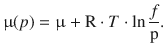
For an ideal gas A, we know that chemical potential at any pressure (![]() ) can be described as per Eq. 2.67:
) can be described as per Eq. 2.67:
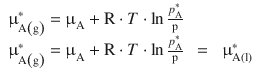
(3.5)
where the asterisks ’*’ indicate the pure component (i.e. here pure component A in either liquid or vapour form).
When two components A and B are mixed, they no longer exist in their pure forms, and we indicate this by omitting the asterisk ’*’. However, for each component A and B in the liquid mixture, the chemical potential in the different phases can still be calculated as in Eq. 3.5; we thus obtain:
![]()
(3.6)
![]()
(3.7)
The pressures pA and pB now indicate the partial pressure of component A and B in the vapour above the liquid.
Inspection of Eqs. 3.5 and 3.6 shows that the chemical potential of component A is different when we compare the pure state with a mixture where A is not the exclusive component of the system. The difference in the chemical potential between both states is available by subtracting Eq. 3.5 from 3.6:
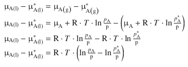
Using the log rule of log b (uv) = log b u + log b v and ![]() (Appendix A.1.2), this yields:
(Appendix A.1.2), this yields:
![]()
which simplifies to
![]()
(3.8)
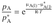
This equation delivers a relationship between the chemical potential of a particular component in a liquid mixture (μA) and its partial vapour pressure (p A). It is found that p A always takes smaller values than ![]() (see next section), which results in
(see next section), which results in ![]() and thus
and thus ![]() ; the chemical potential μ of a solvent is therefore lowered as a result of the presence of the solute.
; the chemical potential μ of a solvent is therefore lowered as a result of the presence of the solute.
3.2.2 Raoult’s Law
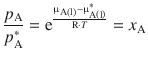
Eq. 3.8 can be transformed with some basic algebra to yield:
(3.9)
The French chemist Francois-Marie Raoult (1830—1901) discovered experimentally that there is a relationship between the partial vapour pressure of component and its mole fraction in the liquid mixture, and summarised his results in 1886 in a rule known as Raoult’s law:
The partial vapour pressure of a component in a liquid mixture is equal to the vapour pressure of the pure component multiplied by its mole fraction in the liquid phase
![]()
(3.10)
Equation 3.9 can thus be extended to read:
(3.9)
Since the mole fraction x A takes values less or up to 1 (0 ≤ x A ≤ 1), an important effect of Raoult’s law is that the vapour pressure of a solution is always lower than that of the pure solvent at any particular temperature. This effect is also known as vapour pressure depression.
Considering that the boiling point of a solution is the temperature at which the vapour pressure of the liquid is equal to the surrounding environmental pressure, another consequence of the above effects is the boiling point elevation observed with liquid solutions. A solution therefore always has a higher boiling point than the pure solvent. More generally, several properties of liquids (T m, T b, p, etc) depend on the presence of solute molecules, in particular the number of particles in solution. Such properties are called colligative properties and will be further discussed in Sect. 4.3.2.
3.2.3 Activity: Mole Fraction for a Non-ideal Solution
In Sect. 2.3.3, we have defined the fugacity f for a non-ideal gas to ensure that the chemical potential of the gas at any pressure can be calculated according to the equation
(2.72)
In Sect. 3.2.1 of this chapter, we established a relationship between the chemical potential of a liquid component (μA(l)) in a mixture and its partial vapour pressure (p A) above the liquid mixture:
![]()
(3.8)
For an ideal ideal solution, it then follows with Raoult’s law that ![]() , and therefore:
, and therefore:
![]()
(3.11)
Analogous to the fugacity in the case of gases, we can now define a property that will account for non-ideal behaviour in the liquid mixtures. This property is called activity (a) and replaces the mole fraction x A in the above case, such that the chemical potential of compound A at any concentration in a non-ideal solution varies as per the relationship:
![]()
(3.12)
The activity coefficient γ indicates the deviation from the ideal behaviour:
![]()
(3.13)
3.2.4 Gibbs Free Energy Change for a Reaction (Part 2)
In Sect. 2.2.5, we discussed the Gibbs free energy change of the following reaction
![]()
by means of the reaction quotient Q, before introducing the chemical potential.
After discussing mixtures of components by means of their chemical potentials in the preceding sections, we can now apply this knowledge and revise our discussion of the Gibbs free energy change for a reaction.
As before, the change in free energy is given by
![]()
This free energy change is an extensive property, as it depends on the actual amounts of compounds. We can introduced the corresponding intensive state functions which are the molar Gibbs free energies (G m):
![]()
The molar Gibbs free energies G m are indeed the chemical potentials, so we can substitute and obtain:
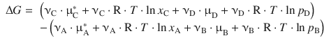
By combining the constant terms (![]() represent the chemical potentials of the components in their pure or standard states), we obtain:
represent the chemical potentials of the components in their pure or standard states), we obtain:
![]()
The constant terms ![]() represent a standard Gibbs free energy change for this reaction and are thus substituted by ΔG —. Using the logarithm rules of a ⋅ log x = log x a , log a + log b = log (a ⋅ b) and
represent a standard Gibbs free energy change for this reaction and are thus substituted by ΔG —. Using the logarithm rules of a ⋅ log x = log x a , log a + log b = log (a ⋅ b) and ![]() (see A.1.2) one obtains:
(see A.1.2) one obtains:
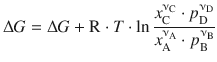
which is a relationship between the Gibbs free energy change for a reaction at varying concentrations of components, here expressed as mole fractions for the liquids A and C, and as partial pressures for the gases B and D. The argument of the logarithm is the reaction coefficient Q introduced earlier. Based on the above rigorous assessment of the chemical potentials, we can thus confirm the relationship introduced in Sect. 2.2.5:
![]()
(2.58)
We recall that when the reaction has reached equilibrium, there is no change the Gibbs free energy observed, therefore:
![]()
Also, at equilibrium, the reaction coefficient Q becomes the equilibrium constant
![]()
One thus obtains from Eq. 2.58 for equilibrium conditions:
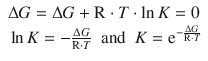
(2.59)
This means that if we can determine the change in the Gibbs free energy of a process, we can calculate the equilibrium constant.