Physical Chemistry Essentials - Hofmann A. 2018
Kinetics
6.6 Linking the Rate Laws with Reaction Mechanisms
So far, we have focused on the explanation of kinetic observations with respect to mathematically formulated rate laws. In the following, we will try to explain the observed rate laws in terms of a postulated reaction mechanism.
6.6.1 Elementary Reactions
Most reactions occur as a sequence of steps which are called elementary reactions, each of which involves only a small number of different molecules or ions (see Sect. 6.1.3).
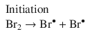
For example, the net reaction describing the formation of HBr from its elements
![]()
can be broken down into the elementary reactions arising from a radical reaction mechanism (Bodenstein and Lind 1907; Christiansen 1967):
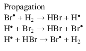
In an elementary reaction, there is no phase specified; it is simply a proposed individual step of a larger reaction mechanism. For instance in the following step
![]()
an H atom attacks a Br2 molecule: a bimolecular reaction. In Sect. 1.3, we introduced the molecularity of the reaction as the number of molecules that come together to react in the elementary reaction. It was also discussed that the molecularity needs to be distinguished from the reaction order which is an empirical quantity, derived from the experimental rate law. However, the reaction order of the individual elementary reactions can be derived directly from the molecularity.
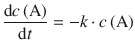
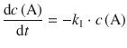
Unimolecular Elementary Reactions
![]()
follow a 1st-order rate law, because the number of molecules A that can decay is proportional to the number of molecules A initially available:
(6.7)
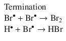
Bimolecular Elementary Reactions
![]()
follow a 2nd-order rate law, because their rate is proportional to the rate with which the two reactants meet—which in turn depends on their concentrations:
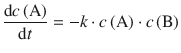
(6.8)
6.6.2 Consecutive Elementary Reactions
When investigating a reaction mechanism, the postulated mechanism can only be explored by a detailed investigation of the system, considering that side products or intermediates may appear in the course of the reaction. Importantly, if a reaction is an elementary bimolecular reaction, then it has a 2nd-order kinetics. However, if 2nd-order kinetics are observed for a net reaction, then it may be a complex reaction.
In the following, we will need to combine a series of consecutive simple steps, i.e. elementary reactions, in order to arrive at a reaction mechanism and the corresponding rate law.
Some reactions proceed through formation of an intermediate (I), so the entire mechanism is described by consecutive unimolecular reactions:
![]()
An example is the decay of radioactive isotopes, such as
![]()
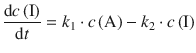
When we consider the variation of concentration with time for consecutive unimolecular reactions, it becomes clear that A decays according to a 1st-order rate law to I:
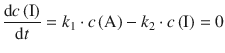
The intermediate I is formed from A, and decays to P; both processes follow 1st-order rate laws:
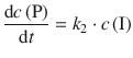
P is formed from I in a 1st-order reaction:
In order to obtain expressions for the concentrations of A, I and P, the differential equations need to be integrated. This yields for the above equations:
![]()
(6.42)
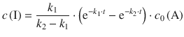
(6.43)
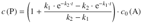
(6.44)
The time-dependent development of the concentrations of A, I and P is illustrated graphically in Fig. 6.15.
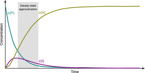
Fig. 6.15
Concentrations of reactant, intermediate and product in a set of consecutive elementary interactions
6.6.3 Steady-State Approximation
It is quite apparent from the algebraic expressions 6.42—6.44 in the previous section, that there is an increase in mathematical complexity when looking at reactions with more than one step. A reaction scheme that comprises many steps may become virtually unsolvable, and numerical rather than algebraic integration may be required.
Alternatively, an approximation can be introduced that yields more directly accessible results than the rigorous mathematical treatment. The (quasi-) steady-state approximation assumes that, after an initial induction period, where concentrations of intermediates rise from zero to a peak value, they remain approximately constant and the rate of change of concentrations of intermediates are negligibly small:
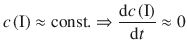
(6.45)
Figure 6.15 shows that this is indeed an approximation as the curve depicting the concentration of the intermediate I does not possess a slope ![]() of zero after rising to a peak value. Nevertheless, we assume the approximation stated by Eq. 6.45 for the following considerations and obtain for the concentration of the intermediate:
of zero after rising to a peak value. Nevertheless, we assume the approximation stated by Eq. 6.45 for the following considerations and obtain for the concentration of the intermediate:
and thus
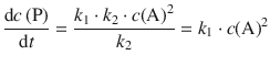
Which yields for the rate of product concentration change:
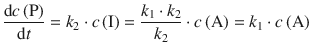
This reveals a 1st-order rate law, whereby P is formed by a decay process of A:
![]()
(6.15)
For the rate of product formation, one thus obtains:
(6.46)
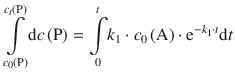
In order to integrate Eq. 6.46, we first isolate the two differential variables on opposite sides of the equation:
![]()
and then consider the development of products in the time interval 0→t, i.e. from c 0(P) to c t (P):
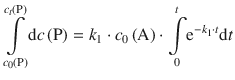
The factors k 1 and c 0(A) are constants with respect to the integral and can thus be taken outside the integral:
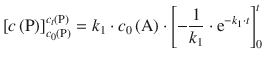
The integral on the left side of the equation is of the type ∫dx = ∫ x 0dx and resolves to x 0 + 1 = x. On the right hand side, the integral is of the type ∫ea ⋅ xdx which resolves to ![]() . We thus obtain:
. We thus obtain:
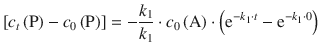
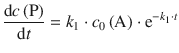
Since there is no product present at time t = 0, it follows that c 0(P) = 0; for the term ![]() , one obtains e0 = 1. Therefore:
, one obtains e0 = 1. Therefore:
![]()
![]()
(6.47)
When compared to the expression we obtained for the product concentration by rigorous kinetic analysis above
(6.44)
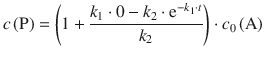
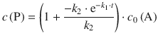
it becomes clear that expression 6.47—obtained with the steady-state approximation—constitutes a special case of Eq. 6.44. In the case when
![]()
k1 in the denominator of the quotient in 6.44can be neglected. Also, a large value of k 2 will give rise to ![]() approaching zero, based on the behaviour of the function e−x (see Fig. 6.16). Under these conditions, Eq. 6.44 becomes:
approaching zero, based on the behaviour of the function e−x (see Fig. 6.16). Under these conditions, Eq. 6.44 becomes:
![]()
and thus shows the relationship (6.47) obtained with the steady-state approximation.
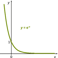
Fig. 6.16
The function e−x anneals to zero when x assumes very large values
It is found that k 2 does not have to be much larger than k 1 in order to obtain reasonably accurate results from the steady-state approximation. For example, k 2 = 20·k 1 already yields a good agreement.
6.6.4 The Rate-Determining Step
In the previous section, we have considered the special case of k 2 ≫ k 1 in the following set of consecutive reactions
![]()
which means that the first reaction proceeds a lot slower than the second reaction. The first reaction thus becomes the rate-determining step.
In consecutive reactions, the rate-determining step is the one with the lowest rate constant. In many cases, the rate law for a consecutive reaction with a rate-determining step can thus be written in a straight-forward way: the rate of the overall reaction equals the rate of the rate-determining step.
6.6.5 Pre-Equilibria
In many instances of consecutive reactions, the first reaction needs to be treated as an equilibrium process ( pre-equilibrium). We thus consider the case where an intermediate I is formed by reaction of A and B in an equilibrium reaction, and that the reaction to the product P proceeds a lot slower than the reverse reaction in the equilibrium:
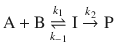
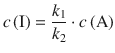
Since we assume the product formation as rate-determining step, the rate constant for the second reaction takes a much smaller value than the rate constant for the reverse reaction of the equilibrium:
![]()
For the first reaction, the equilibrium constant is given by:
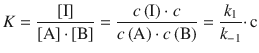
Substituting this into the rate law for the product formation yields:
(6.48)
This is the form of a 2nd-order rate law with the rate constant ![]() .
.
6.6.6 Kinetic and Thermodynamic Control
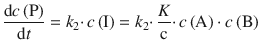
A common feature of reactions in organic chemistry (e.g. nitration of mono-substitute benzenes yielding o-, m-, p-derivatives) is the formation of multiple products from one set of reactants:

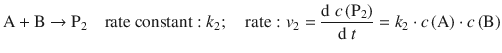
The relative proportion of products formed is given by the ratio of the two rates, and thus the two rate constants:
(6.49)
The ration given by Eq. 6.49 is due to the kinetic control over the proportion of products formed. Notably, this refers to the concentration of products produced at any stage during the reaction, i.e. before the reaction reached equilibrium. Kinetic control is also the reason for the occurrence of electrochemical overpotentials; cf. Sect. 4.2.1). If a reaction is allowed to reach equilibrium, then the proportion of products is determined by the thermodynamic considerations. The ratio is then under thermodynamic control.
6.6.7 The Lindemann—Hinshelwood Mechanism
Examples for unimolecular reactions such as
![]()
are homogeneous gas phase reactions that appear to follow 1st-order kinetics, such as e.g. the isomerisation of cyclo-propane:
![]()
For a 1st-order kinetics, the following rate law can be formulated:
![]()
However, in order to react in this gas phase process, an individual molecule needs to acquire enough energy through collision. Since the collision is a bimolecular process, the question arises how this may still adhere to a kinetic law of 1st-order.
A closer look reveals that there is an elementary unimolecular step in this process (hence 1st-order gas phase reactions are called unimolecular reactions), but there is also a bimolecular step in the overall reaction. Lindemann and Hinshelwood provided a plausible mechanism:
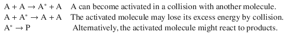
If the unimolecular step of product formation is slow enough to be rate-determining, then the overall reaction will have a 1st-order kinetics (as observed).
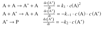
The reaction rates for the above set of elementary reactions can be derived as:
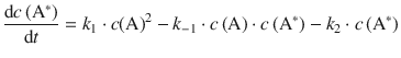
From these individual rates, the net rate of formation of A* is thus:
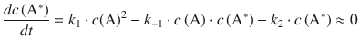
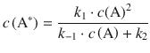
Applying the steady-state approximation, ![]() , yields:
, yields:
This can be re-arranged to:
![]()
which yields for the rate of product formation from this rigorous consideration:
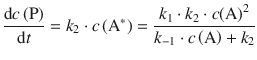
(6.50)
However, this is not a 1st-order rate law!
Two special cases can be singled out. If the overall pressure in the reaction vessel is sufficiently high, the rate of de-activation by collisions between A* and A is greater than the rate of the product formation, then
![]()
![]()
and we can neglect k 2 in the denominator of above product rate and obtain
(6.51)
which describes a rate law for a 1st-order reaction.
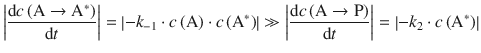
What happens if the overall pressure in this gas phase reaction is lowered, for example by decreasing the concentration of gas A?
If the number of A molecules is decreased, the activation and de-activation reactions are affected. In particular, it becomes less likely that A* molecules are de-activated, since less A molecules are available for a collision. In relation to the de-activation, the product formation step will be more likely. Therefore, at low concentration of A:
![]()
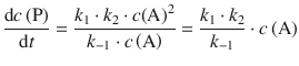
This means we can neglect k −1 ⋅ c(A) in the denominator of Eq. 6.50, and thus obtain:
(6.52)
This means that if we reduce the pressure of A (i.e. the concentration), then the reaction should switch to a 2nd-order rate law, since the activation step becomes rate-determining.
The Lindemann—Hinshelwood mechanism can be experimentally tested, because the 1st-order rate law (Eq. 6.51) was obtained with the assumption that the rate of de-activation by collisions between A* and A is greater than the rate of the product formation. This will only be the case, if there are enough molecules A available for frequent collisions. For the second case of low concentration of A (or, more generally, low overall pressure), a 2nd-order rate law is obtained (Eq. 6.52).