Physical Chemistry Essentials - Hofmann A. 2018
Kinetics
6.9 Reactions in Solution
In the previous chapter, we considered reactions in the gas phase, which proceed by collisional encounter of molecules in space. Reactants in solution are encountering each other in a different way than in the gas-phase.
First, in solution, reactants have to find their way through the solvent (i.e. a network of other molecules), so we can expect the frequency of reactive encounters to be considerably less than in the gas-phase. Second, after an encounter, the reactants are leaving their current positions slower than in the gas phase, since they are held in place by the surrounding solvent. This is called the cage effect.
Conceptually, it is, of course, still required that the reactants require the minimum energy (activation energy), in order for the reaction to proceed. However, an encounter pair may accumulate enough energy to react in due course, even though it may not have had sufficient energy initially. This gives rise to two classes of reactions, namely those with
✵ diffusion control
✵ activation control.
The complicated overall process can be divided into two stages, the encounter step and the post-encounter; both stages can subsequently be combined into the overall rate law.
The Encounter Step
We suppose, the encounter of two reactants was of 1st-order with respect to each of the reactants which need to diffuse towards each other in order to meet up:
![]()
The rate of this step is determined by the constant k d that specifies the diffusional characteristics of A and B.
Post-Encounter
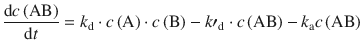
The encounter AB can either break up into its individual partners, or react to product P. If we assume pseudo 1st-order for both processes, we obtain:
![]()
![]()
The rate constant for the break-up is denoted k′d, as this step is the reverse reaction of the encounter step.
Combining Both Steps to Yield the Overall Rate Law
We can thus formulate an expression for the change of concentration of AB over time:
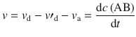
(6.71)
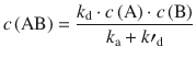
Using the steady-state approximation for intermediates, we can claim:

(6.45)
and thus obtain:
The rate of product formation is thus:
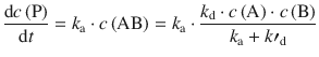
(6.72)
which may be denoted simpler by combining all individual rate constants into an overall rate constant k:
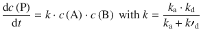
(6.73)
Considering the reaction scheme and the expression of the rate constant in 6.73, we can now distinguish two different cases:
Diffusion Control
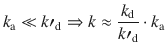
The reaction to product happens faster than the separation of AB. This means, the break-up reaction (characterised by k′d) is much slower than the reaction to product (characterised by k a).
![]()
If k′d is much smaller than k a, k′d has a negligible contribution to the denominator in Eq. 6.73, and can thus be eliminated. This means that the overall rate constant k is dominated by contributions of k d, which is the encounter rate constant. The reaction is then said to be under diffusion control.
Activation Control
In the reverse case, the break-up of AB (characterised by k′d) happens faster then the reaction to product (characterised by k a); k′d is much larger than k a:
If k a is much smaller than k′d, k a has a negligible contribution to the denominator in Eq. 6.73, and can thus be eliminated. This results in an overall rate constant k that is characterised by the encounter equilibrium, but also has contributions from the rate constant that characterises the actual reaction to product. Such reactions are said to be under activation control.