Advanced Calculus of Several Variables (1973)
Part V. Line and Surface Integrals; Differential Forms and Stokes' Theorem
Chapter 2. GREEN'S THEOREM
Let us recall again the fundamental theorem of calculus in the form
![]()
where f is a real-valued ![]() function on the interval [a, b]. Regarding the interval I = [a, b] as an oriented smooth curve from a to b, we may write ∫I df for the left-hand side of (1) . Regarding the right-hand side of (1) as a sort of “0-dimensional integral” of the function f over the boundary ∂I of I (which consists of the two points a and b), and thinking of b as the positive endpoint and a the negative endpoint of I (Fig. 5.9) , let us write
function on the interval [a, b]. Regarding the interval I = [a, b] as an oriented smooth curve from a to b, we may write ∫I df for the left-hand side of (1) . Regarding the right-hand side of (1) as a sort of “0-dimensional integral” of the function f over the boundary ∂I of I (which consists of the two points a and b), and thinking of b as the positive endpoint and a the negative endpoint of I (Fig. 5.9) , let us write
![]()
Then Eq. (1) takes the appealing (if artificially contrived) form
![]()
![]()
Figure 5.9
Green's theorem is a 2-dimensional generalization of the fundamental theorem of calculus. In order to state it in a form analogous to Eq. (2) , we need the notion of the differential of a differential form (to play the role of the differential of a function). Given a ![]() differential form ω = P dx + Q dy in two variables, we define its differential dω by
differential form ω = P dx + Q dy in two variables, we define its differential dω by
![]()
Thus dω is a differential 2-form, that is, an expression of the form a dx dy, where a is a real-valued function of x and y. In a subsequent section we will give a definition of differential 2-forms in terms of bilinear mappings (à la the definition of the differential form a1 dx1 + · · · + an dxn in Section 1 ), but for present purposes it will suffice to simply regard a dx dy as a formal expression whose role is solely notational.
Given a continuous differential 2-form α = a dx dy (that is, the function a is continuous) and a contented set ![]() , the integral of α on D is defined by
, the integral of α on D is defined by
![]()
where the right-hand side is an “ordinary” integral.
Now that we have two types of differential forms, we will refer to
![]()
as a differential 1-form. If moreover we agree to call real-valued functions 0-forms, then the differential of a 0-form is a 1-form, while the differential of a 1-form is a 2-form. We will eventually have a full array of differential forms in all dimensions, with the differential of a k-form being a (k + 1)-form.
We are now ready for a preliminary informal statement of Green's theorem.
Let D be a “nice” region in the plane ![]() 2, whose boundary ∂D consists of a finite number of closed curves, each of which is “positively oriented” with respect to D. If ω = P dx + Q dy is a
2, whose boundary ∂D consists of a finite number of closed curves, each of which is “positively oriented” with respect to D. If ω = P dx + Q dy is a ![]() differential 1-form defined on D, then
differential 1-form defined on D, then
![]()
That is,
Note the formal similarity between Eqs. (2) and (3) . In each, the left-hand side is the integral over a set of the differential of a form, while the right-hand side is the integral of the form over the boundary of the set. We will later see, in Stokes' theorem, a comprehensive multidimensional generalization of this phenomenon.
The above statement fails in several respects to be (as yet) an actual theorem. We have not yet said what we mean by a “nice” region in the plane, nor what it means for its boundary curves to be “positively oriented.” Also, there is a question as to the definition of the integral on the right-hand side of (3) , since we have only defined the integral of a 1-form over a ![]() path (rather than a curve, as such).
path (rather than a curve, as such).
The last question is the first one we will consider. The continuous path γ : [a, b] → ![]() n is called piecewise smooth if there is a partition
n is called piecewise smooth if there is a partition ![]() = {a = a0 < a1 < · · · < ak = b} of the interval [a, b] such that each restriction γi of γ to [ai−1, ai], defined by
= {a = a0 < a1 < · · · < ak = b} of the interval [a, b] such that each restriction γi of γ to [ai−1, ai], defined by
![]()
is smooth. If ω is a continuous differential 1-form, we then define
![]()
It is easily verified that this definition of ∫γ ω is independent of the partition ![]() . (Exercise 2.11) .
. (Exercise 2.11) .
A piecewise-smooth curve C in ![]() n is the image of a piecewise-smooth path γ : [a, b] →
n is the image of a piecewise-smooth path γ : [a, b] → ![]() n which is one-to-one on (a, b); C is closed if γ(a) = γ(b). The path γ is a parametrization of C, and the pair (C, γ) is called an orientedpiecewise-smooth curve [although we will ordinarily abbreviate (C, γ) to C].
n which is one-to-one on (a, b); C is closed if γ(a) = γ(b). The path γ is a parametrization of C, and the pair (C, γ) is called an orientedpiecewise-smooth curve [although we will ordinarily abbreviate (C, γ) to C].
Now let β : [c, d] → ![]() n be a second piecewise-smooth path which is one-to-one on (c, d) and whose image is C. Then we write (C, γ) = (C, β) [respectively, (C, γ) = −(C, β)], and say that γ and β induce the same orientation [respectively, opposite orientations] of C, provided that their unit tangent vectors are equal [respectively, opposite] at each point where both are defined. It then follows from Exercises 1.4 and 1.5 that, for any continuous differential 1-form ω,
n be a second piecewise-smooth path which is one-to-one on (c, d) and whose image is C. Then we write (C, γ) = (C, β) [respectively, (C, γ) = −(C, β)], and say that γ and β induce the same orientation [respectively, opposite orientations] of C, provided that their unit tangent vectors are equal [respectively, opposite] at each point where both are defined. It then follows from Exercises 1.4 and 1.5 that, for any continuous differential 1-form ω,
![]()
if γ and β induce the same orientation of C, while
![]()
if γ and β induce opposite orientations of C (see Exercise 2.12) .
Given an oriented piecewise-smooth curve C, and a continuous differential 1-form ω defined on C, we may now define the integral of ω over C by
![]()
where γ is any parametrization of C. It then follows from (4) and (5) that ∫c ω is thereby well defined, and that
![]()
where C = (C, γ) and − C = − (C, γ) = (C, β), with γ and β inducing opposite orientations.
Now, finally, the right-hand side of (3) is meaningful, provided that ∂D consists of mutually disjoint oriented piecewise-smooth closed curves C1, . . . , Cr; then
![]()
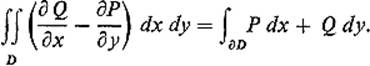
A nice region in the plane is a connected compact (closed and bounded) set ![]() whose boundary ∂D is the union of a finite number of mutually disjoint piecewise-smooth closed curves (as above). It follows from Exercise IV.5.1 that every nice region D is contented, so ∫D α exists if α is a continuous 2-form. Figure 5.10 shows a disk, an annular region (or “disk with one hole”), and a “disk with two holes”; each of these is a nice region.
whose boundary ∂D is the union of a finite number of mutually disjoint piecewise-smooth closed curves (as above). It follows from Exercise IV.5.1 that every nice region D is contented, so ∫D α exists if α is a continuous 2-form. Figure 5.10 shows a disk, an annular region (or “disk with one hole”), and a “disk with two holes”; each of these is a nice region.
It remains for us to say what is meant by a “positive orientation” of the boundary of the nice region D. The intuitive meaning of the statement that an oriented boundary curve C = (C, γ) of a nice region D is positively oriented with respect to D is that the region D stays on one's left as he proceeds around C in the direction given by its parametrization γ. For example, if D is a circular disk, the positive orientation of its boundary circle is its counterclockwise one.
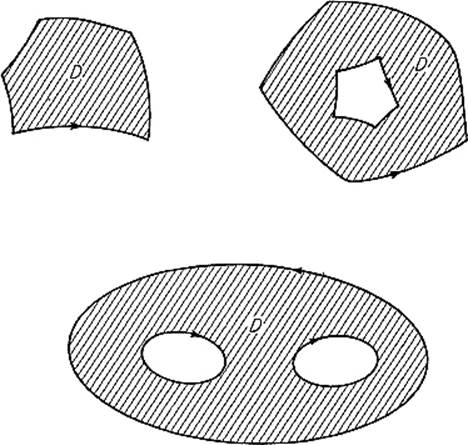
Figure 5.10
According to the Jordan curve theorem, every closed curve C in ![]() 2 separates
2 separates ![]() 2 into two connected open sets, one bounded and the other unbounded (the interior and exterior components, respectively, of
2 into two connected open sets, one bounded and the other unbounded (the interior and exterior components, respectively, of ![]() 2 − C). This is a rather difficult topological theorem whose proof will not be included here. The Jordan curve theorem implies the following fact (whose proof is fairly easy, but will also be omitted): Among all of the boundary curves of the nice region D, there is a unique one whose interior component contains all the other boundary curves (if any) of D. This distinguished boundary curve of D will be called its outer boundary curve; the others (if any) will be called inner boundary curves of D.
2 − C). This is a rather difficult topological theorem whose proof will not be included here. The Jordan curve theorem implies the following fact (whose proof is fairly easy, but will also be omitted): Among all of the boundary curves of the nice region D, there is a unique one whose interior component contains all the other boundary curves (if any) of D. This distinguished boundary curve of D will be called its outer boundary curve; the others (if any) will be called inner boundary curves of D.
The above “left-hand rule” for positively orienting the boundary is equivalent to the following formulation. The positive orientation of the boundary of a nice region D is that for which the outer boundary curve of D is oriented counter-clockwise, and the inner boundary curves of D (if any) are all oriented clockwise.
Although this definition will suffice for our applications, the alert reader will see that there is still a problem—what do the words “clockwise” and “counterclockwise” actually mean? To answer this, suppose, for example, that C is an oriented piecewise-smooth closed curve in ![]() 2 which encloses the origin. Once Green's theorem for nice regions has been proved (in the sense that, given a nice region D, ∫D dω = ∫∂D ω for some orientation of ∂D), it will then follow (see Example 3 below) that
2 which encloses the origin. Once Green's theorem for nice regions has been proved (in the sense that, given a nice region D, ∫D dω = ∫∂D ω for some orientation of ∂D), it will then follow (see Example 3 below) that
![]()
where dθ is the usual polar angle form. We can then say that C is oriented counterclockwise if ∫c dθ = + 2π, clockwise if ∫c dθ = − 2π.
Before proving Green's theorem, we give several typical applications.
Example 1Given a line integral ∫c ω, where C is an oriented closed curve bounding a nice region D, it is sometimes easier to compute ∫D dω. For example,
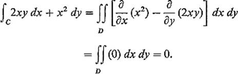
Example 2 Conversely, given an integral ∫∫Df(x, y) dx dy which is to be evaluated, it may be easier to think of a differential 1-form ω such that dω = f(x, y) dx dy, and then compute ∫∂D ω. For example, if D is a nice region and ∂D is positively oriented, then its area is
The formulas
![]()
are obtained similarly. For instance, suppose that D is the elliptical disk ![]() , whose boundary (the ellipse) is parametrized by x = a cos t, y = b sin
, whose boundary (the ellipse) is parametrized by x = a cos t, y = b sin ![]() . Then its area is
. Then its area is
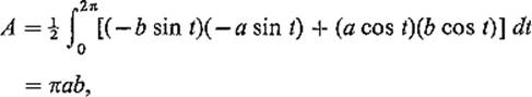
the familiar formula.
Example 3Let C be a piecewise-smooth closed curve in ![]() 2 which encloses the origin, and is oriented counterclockwise. Let Ca be a clockwise-oriented circle of radius a centered at 0, with a sufficiently small that Ca lies in the interior component of
2 which encloses the origin, and is oriented counterclockwise. Let Ca be a clockwise-oriented circle of radius a centered at 0, with a sufficiently small that Ca lies in the interior component of ![]() 2 − C (Fig. 5.11) . Then let D be the annular region bounded by C and Ca. If
2 − C (Fig. 5.11) . Then let D be the annular region bounded by C and Ca. If
![]()
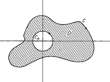
Figure 5.11
then dω = 0 on D (compute it), so
![]()
Since ![]() , by essentially the same computation as in Example 3 of Section 1 , it follows that
, by essentially the same computation as in Example 3 of Section 1 , it follows that
![]()
In particular this is true if C is the ellipse of Exercise 1.12.
On the other hand, if the nice region bounded by C does not contain the origin, then it follows (upon applicaton of Green's theorem to this region) that
![]()
Equation (3) , the conclusion of Green's theorem, can be reformulated in terms of the divergence of a vector field. Given a ![]() vector field F :
vector field F : ![]() n →
n → ![]() n, its divergence div F :
n, its divergence div F : ![]() n →
n → ![]() is the real-valued function defined by
is the real-valued function defined by
![]()
or
![]()
in case n = 2.
Now let ![]() be a nice region with ∂D positively oriented, and let N denote the unit outer normal vector to ∂D, defined as in Exercise 1.20. From that exercise and Green's theorem, we obtain
be a nice region with ∂D positively oriented, and let N denote the unit outer normal vector to ∂D, defined as in Exercise 1.20. From that exercise and Green's theorem, we obtain
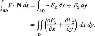
so
![]()
for any ![]() vector field F on D. The number ∫∂D F · N ds is called the flux of the vector field F across ∂D, and it appears frequently in physical applications. If, for example, F is the velocity vector field of a moving fluid, then the flux of F across ∂D measures the rate at which the fluid is leaving the region D.
vector field F on D. The number ∫∂D F · N ds is called the flux of the vector field F across ∂D, and it appears frequently in physical applications. If, for example, F is the velocity vector field of a moving fluid, then the flux of F across ∂D measures the rate at which the fluid is leaving the region D.
Example 4Consider a plane lamina (or thin homogenous plate) in the shape of the open set ![]() , with thermal conductivity k, density ρ, and specific heat c (all constants). Let u(x, y, t) denote the temperature at the point (x, y) at time t. If D is a circular disk in U with boundary circle C, then the heat content of D at time t is
, with thermal conductivity k, density ρ, and specific heat c (all constants). Let u(x, y, t) denote the temperature at the point (x, y) at time t. If D is a circular disk in U with boundary circle C, then the heat content of D at time t is
![]()
Therefore
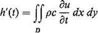
since we can differentiate under the integral sign (see Exercise V.3.5) assuming (as we do) that u is a ![]() function.
function.
On the other hand, since the heat flow vector is −k ![]() u, the total flux of heat across C (the rate at which heat is leaving D) is
u, the total flux of heat across C (the rate at which heat is leaving D) is
![]()
so
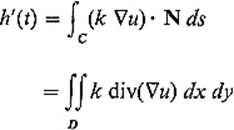
by Eq. (6) .
Equating the above two expressions for h′(t), we find that
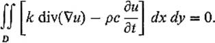
Since D was an arbitrary disk in U, it follows by continuity that
![]()
or
![]()
(where a = ρc/k) at each point of U. Equation (7) is the 2-dimensional heat equation. Under steady state conditions, ∂u/∂t ≡ 0, it reduces to Laplace's equation
![]()
Having illustrated in the above examples the applicability of Green‘s theorem, we now embark upon its proof. This proof depends upon an analysis of the geometry or topology of nice regions, and will proceed in several steps. The first step (Lemma 2.1) is a proof of Green’s theorem for a single nice region—the unit square ![]() ; each of the successive steps will employ the previous one to enlarge the class of those nice regions for which we know that Green's theorem holds.
; each of the successive steps will employ the previous one to enlarge the class of those nice regions for which we know that Green's theorem holds.
Lemma 2.1 (Green's Theorem for the Unit Square) If ω = P dx + Q dy is a ![]() differential 1-form on the unit square I2, and ∂I2 is oriented counter-clockwise, then
differential 1-form on the unit square I2, and ∂I2 is oriented counter-clockwise, then
![]()
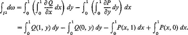
PROOF The proof is by explicit computation. Starting with the left-hand side of (9) , and applying in turn Fubini's theorem and the fundamental theorem of calculus, we obtain
To show that the right-hand side of (9) reduces to the same thing, define the mappings γ1, γ2, γ3, γ4: [0, 1] → ![]() 2 by
2 by
![]()
see Fig. 5.12 . Then
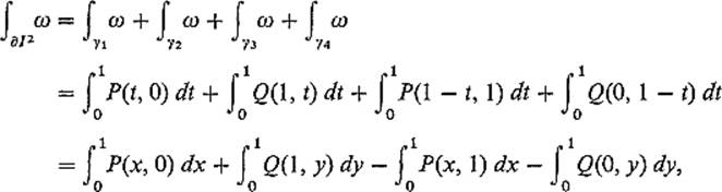
where the last line is obtained from the previous one by means of the substitutions x = t, y = t, x = 1 − t, y = 1 − t, respectively.
![]()
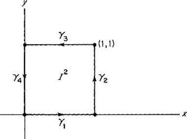
Figure 5.12
Our second step will be to establish Green's theorem for every nice region that is the image of the unit square I2 under a suitable mapping. The set ![]() is called an oriented (smooth) 2-cell if there exists a one-to-one
is called an oriented (smooth) 2-cell if there exists a one-to-one ![]() mapping F: U →
mapping F: U → ![]() 2, defined on a neighborhood U of I2, such that F(I2) = D and the Jacobian determinant of F is positive at each point of U. Notice that the counterclockwise orientation of ∂I2 induces under F an orientation of ∂D(the positive
2, defined on a neighborhood U of I2, such that F(I2) = D and the Jacobian determinant of F is positive at each point of U. Notice that the counterclockwise orientation of ∂I2 induces under F an orientation of ∂D(the positive
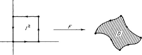
Figure 5.13
or counterclockwise orientation of ∂D). Strictly speaking, an oriented 2-cell should be defined as a pair, consisting of the set D together with this induced orientation of ∂D (Fig. 5.13) . Of course it must be verified that this orientation is well defined; that is, if G is a second one-to-one ![]() mapping such that G(I2) = D and det G′ > 0, then F and G induce the same orientation of ∂D (Exercise 2.13) .
mapping such that G(I2) = D and det G′ > 0, then F and G induce the same orientation of ∂D (Exercise 2.13) .
The vertices (edges) of the oriented 2-cell D are the images under F of the vertices (edges) of the square I2. Since the differential dF: ![]() 2 →
2 → ![]() 2 takes straight lines to straight lines (because it is linear), it follows that the interior angle (between the tangent lines to the incoming and outgoing edges) at each vertex is <π. Consequently ∂D is smooth except at the four vertices, but is not smooth at the vertices. It follows that neither a circular disk nor a triangular one is an oriented 2-cell, since neither has four “vertices” on its boundary. The other region in Fig. 5.14 fails to be an oriented 2-cell because one of its interior angles is >π.
2 takes straight lines to straight lines (because it is linear), it follows that the interior angle (between the tangent lines to the incoming and outgoing edges) at each vertex is <π. Consequently ∂D is smooth except at the four vertices, but is not smooth at the vertices. It follows that neither a circular disk nor a triangular one is an oriented 2-cell, since neither has four “vertices” on its boundary. The other region in Fig. 5.14 fails to be an oriented 2-cell because one of its interior angles is >π.
If the nice region D is a convex quadrilateral—that is, its single boundary curve contains four straight line edges and each interior angle is <π—then it can be shown (by explicit construction of the mapping F) that D is an oriented 2-cell (Exercise 2.14) . More generally it is true that the nice region D is an oriented 2-cell if its single boundary curve consists of exactly four smooth curves, and the interior angle at each of the four vertices is <π (this involves the Jordan curve theorem, and is not so easy).
The idea of the proof of Green‘s theorem for oriented 2-cells is as follows. Given the differential 1-form ω on the oriented 2-cell D, we will use the mapping F: I2 → D to “pull back” ω to a 1-form F*ω (defined below) on I2. We can then apply, to F*ω, Green’s theorem for I2. We will finally verify that the resulting equation ![]() is equivalent to the equation ∫D dω = ∫∂D ω that we are trying to prove.
is equivalent to the equation ∫D dω = ∫∂D ω that we are trying to prove.
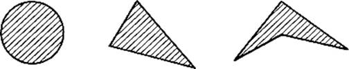
Figure 5.14
Given a ![]() mapping F:
mapping F: ![]() 2 →
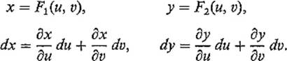
2 → ![]() 2, we must say how differential forms are “pulled back.” It will clarify matters to use uv-coordinates in the domain and xy-coordinates in the image, so
2, we must say how differential forms are “pulled back.” It will clarify matters to use uv-coordinates in the domain and xy-coordinates in the image, so ![]() . A 0-form is just a real valued function φ(x, y), and its pullback is defined by composition,
. A 0-form is just a real valued function φ(x, y), and its pullback is defined by composition,
![]()
That is, F*φ(u, v) = φ(F1(u, v), F2(u, v)), so we are merely using the component functions x = F1(u, v) and y = F2(u, v) of F to obtain by substitution a function of u and v (or 0-form on ![]() ) from the given function φ of x and y.
) from the given function φ of x and y.
Given a 1-form ω = P dx + Q dy, we define its pullback F*ω = F*(ω) under F by
![]()
where
![]()
Formally, we obtain F*(ω) from ω by simply carrying out the substitution
The pullback F*(α) under F of the 2-form α = g dx dy is defined by
![]()
The student should verify as an exercise that F*(α) is the result of making the above formal substitution in α = g dx dy, then multiplying out, making use of the relations du du = dv dv = 0 and dv du = −du dv which were mentioned at the end of Section IV.5. This phenomenon will be explained once and for all in Section 5 of the present chapter.
Example 5Let ![]() be given by
be given by
![]()
so det F′(u, v) ≡ 7. If φ(x, y) = x2 − y2, then
![]()
If ω = −y dx + 2x dy, then
![]()
If α = ex+y dx dy, then
![]()
The following lemma lists the properties of pullbacks that will be needed.
Lemma 2.2 Let F: U → ![]() 2 be as in the definition of the oriented 2-cell D = F(I2). Let ω be a
2 be as in the definition of the oriented 2-cell D = F(I2). Let ω be a ![]() differential 1-form and α a
differential 1-form and α a ![]() differential 2-form on D. Then
differential 2-form on D. Then
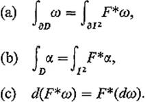
This lemma will be established in Section 5 in a more general context. However it will be a valuable check on the student's understanding of the definitions to supply the proofs now as an exercise. Part (a) is an immediate consequence of Exercise 2.15. Part (b) follows immediately from the change of variables theorem and the definition of F*α (in fact this was the motivation for the definition of F*α). Fact (c), which asserts that the differential operation d “commutes” with the pullback operation F*, follows by direct computation from their definitions.
Lemma 2.3 (Green's Theorem for Oriented 2-Cells) If D is an oriented 2-cell and ω is a ![]() differential 1-form on D, then
differential 1-form on D, then
![]()
PROOF Let D = F(I2) as in the definition of the oriented 2-cell D. Then
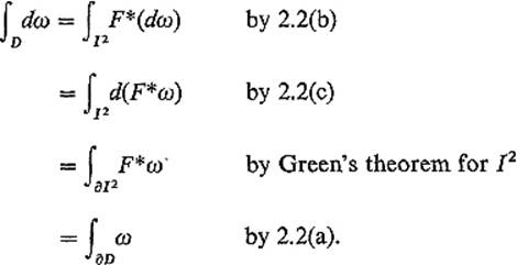
![]()
The importance of Green‘s theorem for oriented 2-cells lies not solely in the importance of oriented 2-cells themselves, but in the fact that a more general nice region D may be decomposable into oriented 2-cells in such a way that the truth of Green’s theorem for each of these oriented 2-cells implies its truth for D. The following examples illustrate this.
Example 6 Consider an annular region D that is bounded by two concentric circles. D is the union of two oriented 2-cells D1 and D2 as indicated in Fig. 5.15.
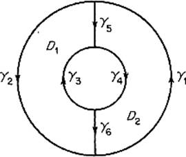
Figure 5.15
In terms of the paths γ1, . . . , γ6 indicated by the arrows, ∂D1 = γ2 − γ6 + γ3 − γ5 and ∂D2 = γ1 + γ5 + γ4 + γ6. Applying Green's theorem to D1 and D2, we obtain
![]()
and
![]()
Upon addition of these two equations, the line integrals over γ5 and γ6 conveniently cancel to give
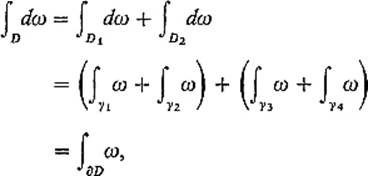
so Green's theorem holds for the annular region D.
Figure 5.16 shows how to decompose a circular or triangular disk D into oriented 2-cells, so as to apply the method of Example 6 to establish Green‘s theorem for D. Upon adding the equations obtained by application of Green’s theorem to each of the oriented 2-cells, the line integrals over the interior segments will cancel because each is traversed twice in opposite directions, leaving as a result Green's theorem for D.
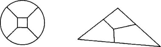
Figure 5.16
Our final version of Green's theorem will result from a formalization of the procedure of these examples. By a (smooth) cellulation of the nice region D is meant a (finite) collection ![]() = {D1, . . . , Dk} of oriented 2-cells such that
= {D1, . . . , Dk} of oriented 2-cells such that
![]()
with each pair of these oriented 2-cells either being disjoint, or intersecting in a single common vertex, or intersecting in a single common edge on which they induce opposite orientations. Given an edge E of one of these oriented 2-cells Di, there are two possibilities. If E is also an edge of another oriented 2-cell Dj of ![]() , then E is called an interior edge. If Di is the only oriented 2-cell of
, then E is called an interior edge. If Di is the only oriented 2-cell of ![]() having E as an edge, then
having E as an edge, then ![]() , and E is a boundary edge. Since ∂D is the union of these boundary edges, the cellulation
, and E is a boundary edge. Since ∂D is the union of these boundary edges, the cellulation ![]() induces an orientation of ∂D. This induced orientation of ∂D is unique—any other cellulation of D induces the same orientation of ∂D (Exercise 2.17) .
induces an orientation of ∂D. This induced orientation of ∂D is unique—any other cellulation of D induces the same orientation of ∂D (Exercise 2.17) .
A cellulated nice region is a nice region D together with a cellulation ![]() of D.
of D.
Theorem 2.4 (Green's Theorem) If ![]() is a cellulated nice region and ω is a
is a cellulated nice region and ω is a ![]() differential 1-form on D, then
differential 1-form on D, then
![]()
PROOF We apply Green's theorem for oriented 2-cells to each 2-cell of the cellulation ![]() = {D1, . . . , Dk}. Then
= {D1, . . . , Dk}. Then
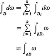
since the line integrals over the interior edges cancel, because each interior edge receives opposite orientations from the two oriented 2-cells of which it is an edge.
![]()
Actually Theorem 2.4 suffices to establish Green's theorem for all nice regions because every nice region can be cellulated. We refrain from stating this latter result as a formal theorem, because it is always clear in practice how to cellulate a given nice region, so that Theorem 2.4 applies. However an outline of the proof would go as follows. Since we have seen how to cellulate triangles, it suffices to show that every nice region can be “triangulated,” that is, decomposed into smooth (curvilinear) triangles that intersect as do the 2-cells of a cellulation. If D has a single boundary curve with three or more vertices, it suffices to pick an interior point p of D, and then join it to the vertices of ∂D with smooth curves that intersect only in p (as in Fig. 5.17) . Proceeding by
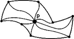
Figure 5.17
induction on the number n of boundary curves of the nice region D, we then notice that, if n > 1, D can be expressed as the union of an oriented 2-cell D1 and a nice region D2 having n − 1 boundary curves (Fig. 5.18) . By induction, D1 and D2 can then both be triangulated.
This finally brings us to the end of our discussion of the proof of Green's theorem. We mention one more application.
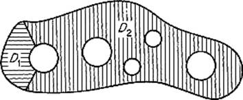
Figure 5.18
Theorem 2.5 If ω = P dx + Q dy is a ![]() differential 1-form defined on
differential 1-form defined on ![]() 2, then the following three conditions are equivalent:
2, then the following three conditions are equivalent:
(a)There exists a function f : ![]() 2 →
2 → ![]() such that df = ω.
such that df = ω.
(b)∂Q/∂x = ∂P/∂y on ![]() 2.
2.
(c)Given points a and b, the integral ∫γ ω is independent of the piecewise smooth path γ from a to b.
PROOF We already know that (a) implies both (b) and (c) (Corollary 1.6), so it suffices to show that both (b) and (c) imply (a). Given ![]() define
define
![]()
where γ(x, y) is the straight-line path from (0, 0) to (x, y) (see Fig. 5.19) .
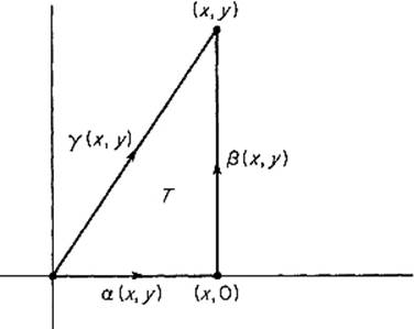
Figure 5.19
Let α(x, y) be the straight-line path from (0, 0) to (x, 0), and β(x, y) the straight-line path from (x, 0) to (x, y). Then either immediately from (c), or by application of Green's theorem to the triangle T if we are assuming (b), we see that
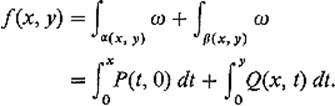
Therefore
![]()
by the fundamental theorem of calculus. Similarly ∂f/∂x = P, so df = ω.
![]()
The familiar form dθ shows that the plane ![]() 2 in Theorem 2.5 cannot be replaced by an arbitrary open subset U. However it suffices (as we shall see in Section 8) for U to be star shaped, meaning that U contains the segment γ(x, y), for every
2 in Theorem 2.5 cannot be replaced by an arbitrary open subset U. However it suffices (as we shall see in Section 8) for U to be star shaped, meaning that U contains the segment γ(x, y), for every ![]()
Example 7If ω = y dx + x dy, then the function f defined by (10) is given by
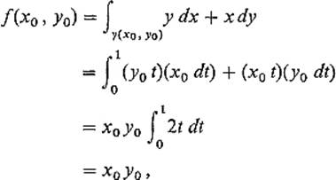
so f(x, y) = xy (as, in the example, could have been seen by inspection).
Exercises
2.1Let C be the unit circle x2 + y2 = 1, oriented counterclockwise. Evaluate the following line integrals by using Green's theorem to convert to a double integral over the unit disk D:
(a) ∫c (3x2 − y) dx + (x + 4y3) dy,
(b) ∫c (x2 + y2) dy.
2.2Parametrize the boundary of the ellipse ![]() and then use the formula
and then use the formula ![]() to compute its area.
to compute its area.
2.3Compute the area of the region bounded by the loop of the “folium of Descartes,” x3 + y3 = 3xy. Hint: Compute the area of the shaded half D (Fig. 5.20) . Set y = tx to discover a parametrization of the curved part of ∂D.
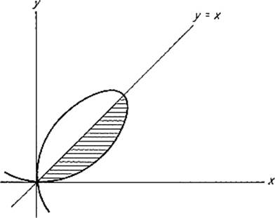
Figure 5.20
2.4Apply formula (10) in the proof of Theorem 2.5 to find a potential function φ (such that ![]() φ = F) for the vector field F :
φ = F) for the vector field F : ![]() 2 →
2 → ![]() 2, if
2, if
(a) F(x, y) = (2xy3, 3x2y2),
(b) F(x, y) = (sin 2x cos2 y, −sin2 x sin 2y).
2.5Let f, g : [a, b] → ![]() be two
be two ![]() functions such that f(x) > g(x) > 0 on [a, b]. Let D be the nice region that is bounded by the graphs y = f(x), y = g(x) and the vertical lines x = a, x = b. Then the volume, of the solid obtained by revolving D about the x-axis, is
functions such that f(x) > g(x) > 0 on [a, b]. Let D be the nice region that is bounded by the graphs y = f(x), y = g(x) and the vertical lines x = a, x = b. Then the volume, of the solid obtained by revolving D about the x-axis, is
![]()
by Cavalieri's principle (Theorem IV.4.2) . Show first that
![]()
Then apply Green's theorem to conclude that
![]()
where A is the area of the region D, and ![]() is the y-coordinate of its centroid (see Exercise IV.5.16) .
is the y-coordinate of its centroid (see Exercise IV.5.16) .
2.6Let f and g be ![]() functions on an open set containing the nice region D, and denote by N the unit outer normal vector to ∂D (see Exercise 1.20). The Laplacian
functions on an open set containing the nice region D, and denote by N the unit outer normal vector to ∂D (see Exercise 1.20). The Laplacian ![]() 2f and the normal derivative ∂f/∂n are defined by
2f and the normal derivative ∂f/∂n are defined by
![]()
Prove Green's formulas:
(a) ![]()
(b) 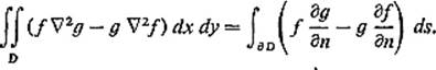
Hint: For (a) apply Green's theorem with P = − f ∂g/∂y and Q = f ∂g/∂x.
2.7If f is harmonic on D, that is, ![]() 2f ≡ 0, set f = g in Green's first formula to obtain
2f ≡ 0, set f = g in Green's first formula to obtain
![]()
If f ≡ 0 on ∂D, conclude that f ≡ 0 on D.
2.8Suppose that f and g both satisfy Poisson's equation on D, that is,
![]()
where φ(x, y) is given on D. If f = g on ∂D, apply the previous exercise to f − g, to conclude that f = g on D. This is the uniqueness theorem for solutions of Poisson's equation.
2.9Given ![]() , let F :
, let F : ![]() 2 − p →
2 − p → ![]() 2 be the vector field defined by
2 be the vector field defined by
![]()
If C is a counterclockwise circle centered at p, show by direct computation that
![]()
2.10Let C be a counterclockwise-oriented smooth closed curve enclosing the points p1, . . . , pk. If F is the vector field defined for x ≠ pi by
![]()
where q1, . . . , qk are constants, deduce from the previous exercise that
![]()
Hint: Apply Green's theorem on the region D which is bounded by C and small circles centered at the points p1, . . . , pk.
2.11Show that the integral ∫α ω, of the differential form ω over the piecewise-smooth path γ is independent of the partition ![]() used in its definition.
used in its definition.
2.12If α and β induce opposite orientations of the piecewise-smooth curve, show that ∫α ω = − ∫β ω.
2.13Prove that the orientation of the boundary of an oriented 2-cell is well-defined.
2.14Show that every convex quadrilateral is a smooth oriented 2-cell.
2.15If the mapping γ : [a, b] → ![]() 2 is
2 is ![]() and ω is a continuous 1-form, show that
and ω is a continuous 1-form, show that
![]()
2.16Prove Lemma 2.2.
2.17Prove that the orientation of the boundary of a cellulated nice region is well-defined.