Calculus For Dummies, 2nd Edition (2014)

Part V. Integration and Infinite Series

IN THIS PART …

The meaning of integration: Integration is basically just fancy calculus addition. It works by sort of slicing up something into tiny bits (actually infinitesimal bits) and then adding up the bits to get the total. This allows you to find the total of things — say, the total volume of some weird bell-shaped object — that can’t be handled by simple, pre-calculus formulas.

The fundamental theorem of calculus: Integration is basically differentiation in reverse — namely, antidifferentiation. There’s an intimate yin/yang connection between integration and differentiation which this part looks at from several angles.

Techniques for calculating antiderivatives: Substitution, integration by parts, trig integrals, and partial fractions.

Integration word problems: Calculating the area between curves, finding volume with the washer method, computing arc length and surface area, and improper integrals.

L’Hôpital’s rule: A nice trick for solving limit problems.

Taming infinity: Ten tests for the convergence or divergence of infinite series.

Chapter 14. Intro to Integration and Approximating Area

IN THIS CHAPTER

Integrating — adding it all up

Approximating areas and sizing up sigma sums

Using the definite integral to get exact areas

Totaling up trapezoids

Simpson’s rule: Calculus for Bart and Homer

Since you’re still reading this book, I presume that means you survived differentiation (Chapters 9 through 13). Now you begin the second major topic in calculus: integration. Just as two simple ideas lie at the heart of differentiation — rate (like miles per hour) and the steepness or slope of a curve — integration can also be understood in terms of two simple ideas — adding up small pieces of something and the area under a curve. In this chapter, I introduce you to these two fundamental concepts.

Integration: Just Fancy Addition

Consider the lamp on the left in Figure 14-1. Say you want to determine the volume of the lamp’s base. Why would you want to do that? Beats me. Anyway, a formula for the volume of such a weird shape doesn’t exist, so you can’t calculate the volume directly.

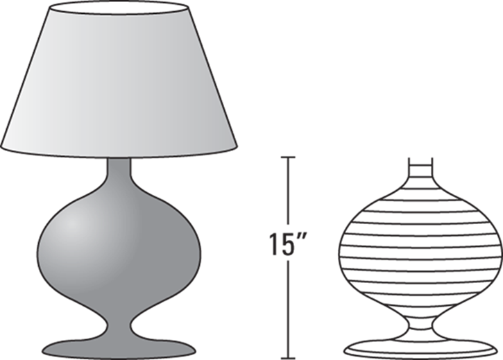
FIGURE 14-1: A lamp with a curvy base and the base cut into thin horizontal slices.

You can, however, calculate the volume with integration. Imagine that the base is cut up into thin, horizontal slices as shown on the right in Figure 14-1.

Can you see that each slice is shaped like a thin pancake? Now, because there is a formula for the volume of a pancake (a pancake is just a very short cylinder), you can determine the total volume of the base by simply calculating the volume of each pancake-shaped slice and then adding up the volumes. That’s integration in a nutshell.

But, of course, if that’s all there was to integration, there wouldn’t be such a fuss about it — certainly not enough to vault Newton, Leibnitz, and the other all-stars into the mathematics hall of fame. What makes integration one of the great achievements in the history of mathematics is that — to continue with the lamp example — it gives you the exact volume of the lamp’s base by sort of cutting it into an infinite number of infinitely thin slices. Now that is something. If you cut the lamp into fewer than an infinite number of slices, you can get only a very good approximation of the total volume — not the exact answer — because each pancake-shaped slice would have a weird, curved edge which would cause a small error when computing the volume of the slice with the cylinder formula.

Integration has an elegant symbol: . You’ve probably seen it before — maybe in one of those cartoons with some Einstein guy in front of a blackboard filled with indecipherable gobbledygook. Soon, this will be you. That’s right: You’ll be filling up pages in your notebook with equations containing the integration symbol. Onlookers will be amazed and envious.

You can think of the integration symbol as just an elongated S for “sum up.” So, for our lamp problem, you can write

where dB means a little bit of the base — actually an infinitely small piece. So the equation just means that if you sum up all the little pieces of the base from the bottom to the top, the result is B, the volume of the whole base.

This is a bit oversimplified — I can hear the siren of the math police now — but it’s a good way to think about integration. By the way, thinking of dB as a little or infinitesimal piece of B is an idea you saw before with differentiation (see Chapter 9), where the derivative or slope, , is equal to the ratio of a little bit of y to a little bit of x, as you shrink the stair step down to an infinitesimal size (see Figure 9-13). Thus, both differentiation and integration involve infinitesimals.

So, whenever you see something like

it just means that you add up all the little (infinitesimal) pieces of the mumbo jumbo from a to b to get the total of all of the mumbo jumbo from a to b. Or you might see something like

which means to add up the little pieces of distance traveled between 0 and 20 seconds to get the total distance traveled during that time span.

To sum up — that’s a pun! — the mathematical expression to the right of the integration symbol stands for a little bit of something, and integrating such an expression means to add up all the little pieces between some starting point and some ending point to determine the total between the two points.

Finding the Area Under a Curve

As I discuss in Chapter 9, the most fundamental meaning of a derivative is that it’s a rate, a this per that like miles per hour, and that when you graph the this as a function of the that (like miles as a function of hours), the derivative becomes the slope of the function. In other words, the derivative is a rate, which on a graph appears as a slope.

It works in a similar way with integration. The most fundamental meaning of integration is to add up (you might be adding up distances or volumes, for example). And when you depict integration on a graph, you can see the adding up process as a summing up of little bits of area to arrive at the total area under a curve. Consider Figure 14-2.

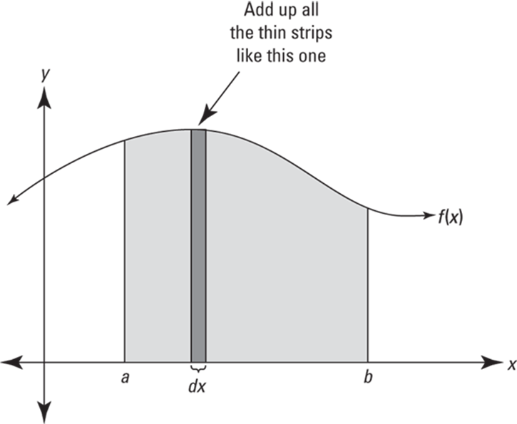
FIGURE 14-2: Integrating from to means finding the area under the curve between a and b.

The shaded area in Figure 14-2 can be calculated with the following integral:

Look at the thin rectangle in Figure 14-2. It has a height of and a width of dx (a little bit of x), so its area (length times width, of course) is given by . The above integral tells you to add up the areas of all the narrow rectangular strips between a and b under the curve . As the strips get narrower and narrower, you get a better and better estimate of the area. The power of integration lies in the fact that it gives you the exact area by sort of adding up an infinite number of infinitely thin rectangles.

If you’re doing a problem where both the x and y axes are labeled in a unit of length, say, feet, then each thin rectangle measures so many feet by so many feet, and its area — length times width — is some number of square feet. In this case, when you integrate to get the total area under the curve between a and b, your final answer will be an amount of — what else? — area. But you can use this adding-up-areas-of-rectangles scheme to add up tiny bits of anything — distance, volume, or energy, for example. In other words, the area under the curve doesn’t have to stand for an actual area.

If, for example, the units on the x-axis are hours and the y-axis is labeled in miles per hour, then, because rate times time equals distance (and because ), the area of each rectangle represents an amount of distance (in miles), and the total area gives you the total distance traveled during the given time interval. Or if the x-axis is labeled in hours and the y-axis in kilowatts of electrical power — in which case the curve gives power usage as a function of time — then the area of each rectangular strip (kilowatts times hours) represents a number of kilowatt-hours of energy. In that case, the total area under the curve gives you the total number of kilowatt-hours of energy consumption between two points in time.

Figure 14-3 shows how you would do the lamp volume problem — from earlier in this chapter — by adding up areas. In this graph, the function gives the cross-sectional area of a thin pancake slice of the lamp as a function of its height measured from the bottom of the lamp. So this time, the h-axis is labeled in inches (that’s h as in height from the bottom of the lamp), and the y-axis is labeled in square inches, and thus each thin rectangle has a width measured in inches and a height measured in square inches. Its area, therefore, represents inches times square inches, or cubic inches of volume.

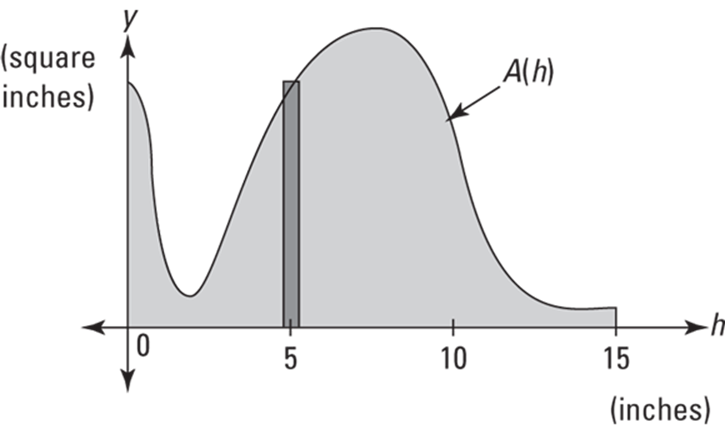
FIGURE 14-3: This shaded area gives you the volume of the base of the lamp in Figure 14-1.

The area of the thin rectangle in Figure 14-3 represents the volume of the thin pancake slice of the lamp 5 inches up from the bottom of the base. The total shaded area and thus the volume of the lamp’s base is given by the following integral:

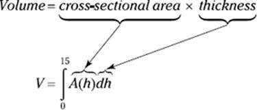
This integral tells you to add up the volumes of all the thin pancake slices from 0 to 15 inches (that is, from the bottom to the top of the lamp’s base), each slice having a volume given by (its cross-sectional area) times dh(its height or thickness). (By the way, Figure 14-3 resembles the left half of the lamp’s base (tilted on its side), but it’s not that. It has a similar shape because where the lamp base is wide, the corresponding circular slice has a large area.)

Okay, enough of this introductory stuff. In the next section, you actually calculate some areas.

Approximating Area

Before explaining how to calculate exact areas, I want to show you how to approximate areas. The approximation method is useful not only because it lays the groundwork for the exact method — integration — but because for some curves, integration is impossible, and an approximation of area is the best you can do.

Approximating area with left sums

Say you want the exact area under the curve between and . See the shaded area on the graph on the left in Figure 14-4.

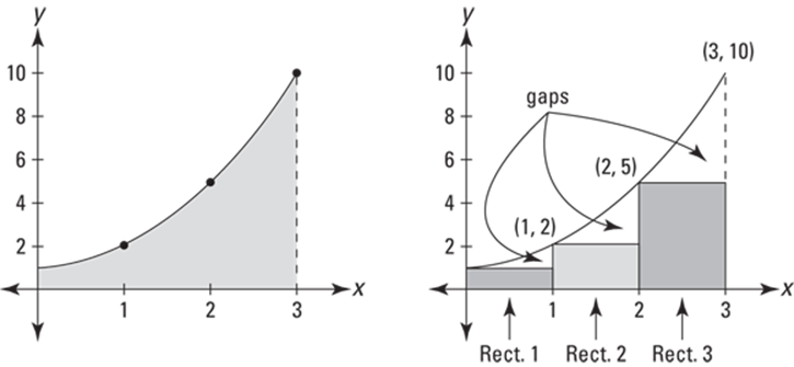
FIGURE 14-4: The exact area under between and  (left) is approximated by the area of three rectangles (right).

You can get a rough estimate of the total area by drawing three rectangles under the curve, as shown on the right in Figure 14-4, and then adding up their areas.

The rectangles in Figure 14-4 represent a so-called left sum because the height of each rectangle is determined by where the upper left corner of each rectangle touches the curve. Each rectangle has a width of 1 and the height of each is given by the height of the function at the rectangle’s left edge. So, rectangle number 1 has a height of ; its area is thus , or 1. Rectangle 2 has a height of , so its area is , or 2. And rectangle 3 has a height of , so its area is , or 5. Adding these three areas gives you a total of , or 8. You can see that this is an underestimate of the total area under the curve because of the three gaps between the rectangles and the curve shown in Figure 14-4.

For a better estimate, double the number of rectangles to six. Figure 14-5 shows six “left” rectangles under the curve and also how the six rectangles begin to fill up the three gaps you see in Figure 14-4.

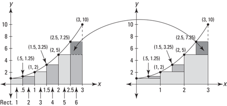
FIGURE 14-5: Six “left” rectangles approximate the area under

See the three small shaded rectangles in the graph on the right in Figure 14-5? They sit on top of the three rectangles from Figure 14-4 and represent how much the area estimate has improved by using six rectangles instead of three.

Now total up the areas of the six rectangles. Each has a width of 0.5 and the heights are and so on. I’ll spare you the arithmetic. Here’s the total: . This is a better estimate, but it’s still an underestimate because of the six small gaps you can see on the left graph in Figure 14-5.

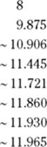
Table 14-1 shows the area estimates given by 3, 6, 12, 24, 48, 96, 192, and 384 rectangles. You don’t have to double the number of rectangles each time like I’ve done here. You can use any number of rectangles of equal width that you want. I just like the doubling scheme because, with each doubling, the gaps are plugged up more and more in the way shown in Figure 14-5. Any guesses as to where the estimates in Table 14-1 are headed? Looks like 12 to me.

TABLE 14-1 Estimates of the Area Under  Given by Increasing Numbers of “Left” Rectangles

Here’s the fancy-pants formula for a left-rectangle sum:

The left rectangle rule: You can approximate the exact area under a curve between a and b, , with a sum of left rectangles of equal width given by the following formula. In general, the more rectangles, the better the estimate.

where n is the number of rectangles, is the width of each rectangle, through are the x-coordinates of the left edges of the n rectangles, and the function values are the heights of the rectangles.

I’d better explain this formula a bit. Look back to the six rectangles shown in Figure 14-5. The width of each rectangle equals the length of the total span from 0 to 3 (which of course is , or 3) divided by the number of rectangles, 6. That’s what the does in the formula.

Now, what about those xs with the subscripts? The x-coordinate of the left edge of rectangle 1 in Figure 14-5 is called , the right edge of rectangle 1 (which is the same as the left edge of rectangle 2) is at , the right edge of rectangle 2 is at , the right edge of rectangle 3 is at , and so on all the way up to the right edge of rectangle 6, which is at . For the six rectangles in Figure 14-5, is 0, is 0.5, is 1, is 1.5, is 2, is 2.5, and is 3. The heights of the six left rectangles in Figure 14-5 occur at their left edges, which are at through . You don’t use the right edge of the last rectangle, , in a left sum. That’s why the list of function values in the formula stops at . This all becomes clearer — cross your fingers — when you look at the formula for right rectangles in the next section.

Here’s how to use the formula for the six rectangles in Figure 14-5:

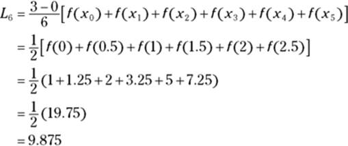
Note that had I distributed the width of to each of the heights after the third line in the solution, you’d have seen the sum of the areas of the six rectangles — which you saw two paragraphs below Figure 14-5. The formula just uses the shortcut of first adding up the heights and then multiplying by the width.

Approximating area with right sums

Now estimate the same area under from 0 to 3 with right rectangles. This method works like the left sum method except each rectangle is drawn so that its right upper corner touches the curve. See Figure 14-6.

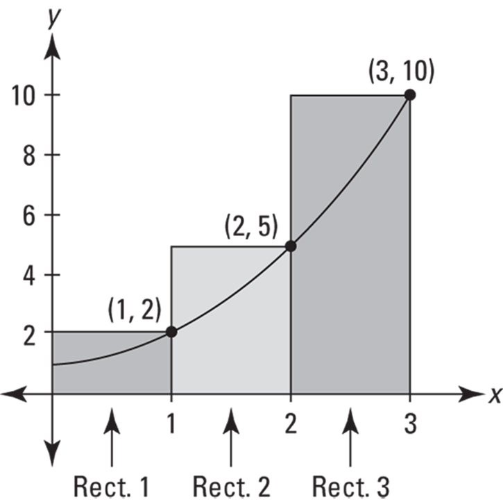
FIGURE 14-6: Three right rectangles used to approximate the area under  .

The heights of the three rectangles in Figure 14-6 are given by the function values at their right edges: , , and . Each rectangle has a width of 1, so the areas are 2, 5, and 10, which total 17. You don’t have to be a rocket scientist to see that this time you get an overestimate of the actual area under the curve, as opposed to the underestimate that you get with the left-rectangle method I detail in the previous section (more on that in a minute). Table 14-2 shows the improving estimates you get with more and more right rectangles.

TABLE 14-2 Estimates of the Area Under  Given by Increasing Numbers of “Right” Rectangles

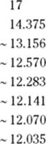
Looks like these estimates are also headed toward 12. Here’s the formula for a right rectangle sum.

The right rectangle rule: You can approximate the exact area under a curve between a and b, , with a sum of right rectangles given by the following formula. In general, the more rectangles, the better the estimate.

where n is the number of rectangles, is the width of each rectangle, through are the x-coordinates of the right edges of the n rectangles, and the function values are the heights of the rectangles.

If you compare this formula to the one for a left rectangle sum, you get the complete picture about those subscripts. The two formulas are the same except for one thing. Look at the sums of the function values in both formulas. The right sum formula has one value, , that the left sum formula doesn’t have, and the left sum formula has one value, , that the right sum formula doesn’t have. All the function values between those two appear in both formulas. You can get a better handle on this by comparing the three left rectangles from Figure 14-4 to the three right rectangles from Figure 14-6. Their areas and totals, which we earlier calculated, are

The values used in the sums of the areas are the same except for the left-most left rectangle value and the right-most right rectangle value. Both sums include rectangles with areas 2 and 5. If you look at how the rectangles are constructed, you can see that the second and third rectangles in Figure 14-4 are the same as the first and second rectangles in Figure 14-6.

Approximating area with midpoint sums

A third way to approximate areas with rectangles is to make each rectangle cross the curve at the midpoint of its top side. A midpoint sum is usually a much better estimate of area than either a left or a right sum. Figure 14-7shows why.

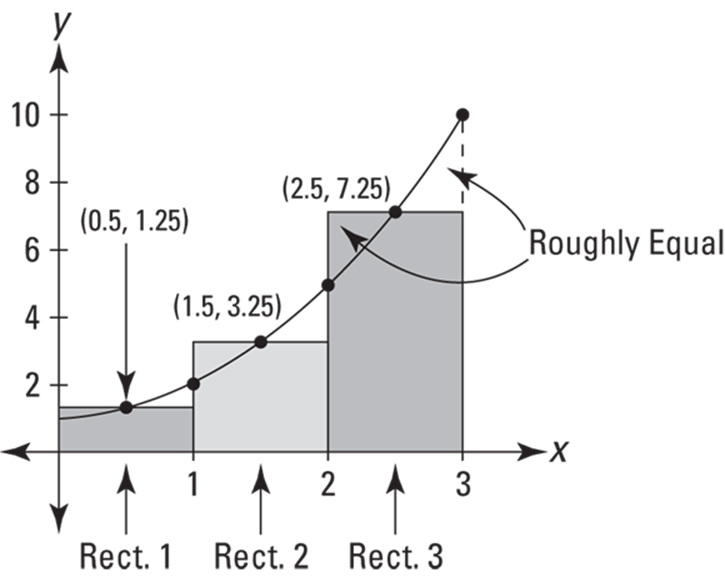
FIGURE 14-7: Three midpoint rectangles give you a much better estimate of the area under

You can see in Figure 14-7 that the part of each rectangle that’s above the curve looks about the same size as the gap between the rectangle and the curve. A midpoint sum produces such a good estimate because these two errors roughly cancel out each other.

For the three rectangles in Figure 14-7, the widths are 1 and the heights are, , and . The total area comes to 11.75. Table 14-3 lists the midpoint sums for the same number of rectangles used in Tables 14-1 and 14-2.

TABLE 14-3 Estimates of the Area Under  Given by Increasing Numbers of “Midpoint” Rectangles

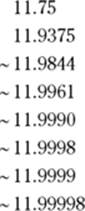
If you had any doubts that the left and right sums in Tables 14-1 and 14-2 were heading to 12, Table 14-3 should dispel them. Spoiler alert: Yes, in fact, the exact area is 12. (I show you how to calculate that in about 5 or 6 pages.) And to see how much faster the midpoint approximations approach the exact answer of 12 than the left or right approximations, compare the three tables. The error with 6 midpoint rectangles is about the same as the error with 192 left or right rectangles!

Here’s the mumbo jumbo.

The midpoint rule: You can approximate the exact area under a curve between a and b, , with a sum of midpoint rectangles given by the following formula. In general, the more rectangles, the better the estimate.

where n is the number of rectangles, is the width of each rectangle, through are the evenly spaced points from a to b, and the function values are the heights of the rectangles.

Definition of Riemann sum: All three sums — left, right, and midpoint — are called Riemann sums, after the great German mathematician Bernhard Riemann (1826-66). Basically, any approximating sum made up of rectangles is a Riemann sum, including weird sums consisting of rectangles of unequal width. Luckily, you won’t have to deal with those in this book or your calculus course.

The left, right, and midpoint sums in Tables 14-1, 14-2, and 14-3 are all heading toward 12, and if you could slice up the area into an infinite number of rectangles, you’d get the exact area of 12. But I’m getting ahead of myself.

Getting Fancy with Summation Notation

Before I get to the formal definition of the definite integral — that’s the incredible calculus tool that sort of cuts up an area into an infinite number of rectangles and thereby gives you the exact area — there’s one more thing to take care of: summation notation.

Summing up the basics

For adding up long series of numbers like the rectangle areas in a left, right, or midpoint sum, summation or sigma notation comes in handy. Here’s how it works. Say you wanted to add up the first 100 multiples of 5 — that’s from 5 to 500. You could write out the sum like this:

But with sigma notation (sigma, is the 18th letter of the Greek alphabet) the sum is much more condensed and efficient, and, let’s be honest, it looks pretty cool:

This notation just tells you to plug 1 in for the i in 5i, then plug 2 into the i in 5i, then 3, then 4, and so on, up to 100. Then you add up the results. So that’s plus plus and so on, up to . This produces the same thing as writing out the sum the long way. By the way, the letter i has no significance. You can write the sum with a j, , or any other letter.

Here’s one more. If you want to add up , you can write the sum with sigma notation as follows:

There’s really nothing to it.

Writing Riemann sums with sigma notation

You can use sigma notation to write out the right-rectangle sum for the curve we’ve been looking at. By the way, you don’t need sigma notation for the math that follows. It’s just a “convenience” — oh, sure. Cross your fingers and hope your teacher decides not to cover this. It gets pretty gnarly.

Recall the formula for a right sum from the earlier “Approximating area with right sums” section:

Here’s the same formula written with sigma notation:

(Note that I could have written this instead as , which would have more nicely mirrored the above formula where the is on the outside. Either way is fine — they’re equivalent — but I chose to keep the on the inside so that the sum is actually a sum of rectangles. In other words, with the on the inside, the expression after the symbol, , which the symbol tells you to add up, is the area of each rectangle, namely height times base.)

Now work this out for the six right rectangles in Figure 14-8.

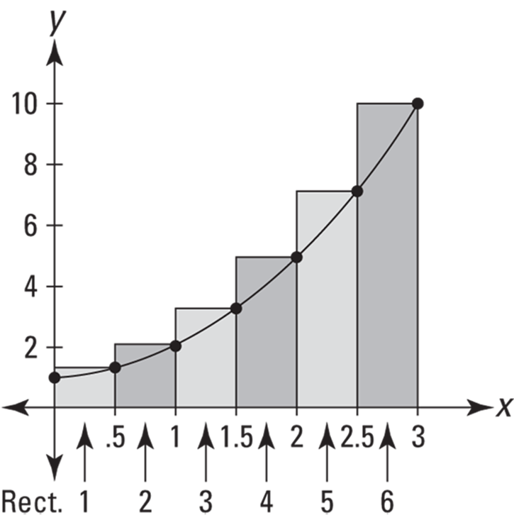
FIGURE 14-8: Six right rectangles approximate the area under between 0 and 3.

You’re figuring the area under between and with six rectangles, so the width of each, , is , or , or . So now you’ve got

Next, because the width of each rectangle is , the right edges of the six rectangles fall on the first six multiples of : 0.5, 1, 1.5, 2, 2.5, and 3. These numbers are the x-coordinates of the six points through ; they can be generated by the expression , where i equals 1 through 6. You can check that this works by plugging 1 in for i in , then 2, then 3, up to 6. So now you can replace the in the formula with , giving you

Our function, , is so , and so now you can write

If you plug 1 into i, then 2, then 3, and so on up to 6 and do the math, you get the sum of the areas of the rectangles in Figure 14-8. This sigma notation is just a fancy way of writing the sum of the six rectangles.

Are we having fun? Hold on, it gets worse — sorry. Now you’re going to write out the general sum for an unknown number, n, of right rectangles. The total span of the area in question is 3, right? You divide this span by the number of rectangles to get the width of each rectangle. With 6 rectangles, the width of each is ; with n rectangles, the width of each is . And the right edges of the n rectangles are generated by , for i equals 1 through n. That gives you

Or, because ,

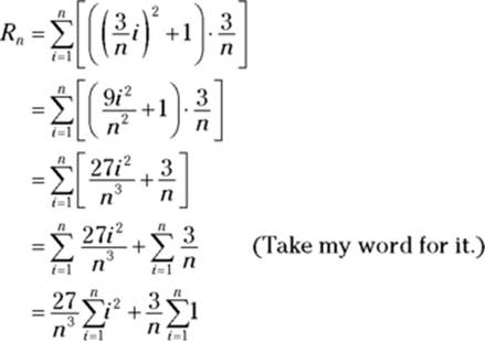
For this last step, you pull the and the through the summation symbols — you’re allowed to pull out anything except for a function of i, the so-called index of summation. Also, the second summation in the last step has just a 1 after it and no i. So there’s nowhere to plug in the values of i. This situation may seem a bit weird, but all you do is add up n 1s, which equals n (I do this below).

You’ve now arrived at a critical step. With a sleight of hand, you’re going to turn the above Riemann sum into a formula in terms of n. (This formula is what you use in the next section to obtain the exact area under the curve.)

Now, as almost no one knows, the sum of the first n square numbers, , equals . (By the way, this 6 has nothing to do with the fact that we used 6 rectangles a couple pages back.) So, you can substitute that expression for the in the last line of the sigma notation solution, and at the same time substitute n for :

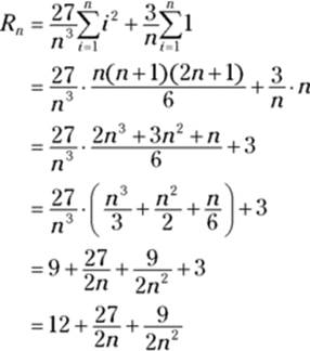
The end. Finally! This is the formula for the area of n right rectangles between and under the function . You can use this formula to produce the approximate areas given in Table 14-2. But once you’ve got such a formula, it’d be kind of pointless to produce a table of approximate areas, because you can use the formula to determine the exact area. And it’s a snap. I get to that in a minute in the next section.

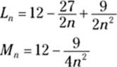
But first, here are the formulas for n left rectangles and n midpoint rectangles between and under the same function, . These formulas generate the area approximations in Tables 14-1 and 14-3. The algebra for deriving these formulas is even worse than what you just did for the right rectangle formula, so I decided to skip it. Do you mind? I didn’t think so.

And now, what you’ve all been waiting for …

Finding Exact Area with the Definite Integral

Having laid all the necessary groundwork, you’re finally ready to move on to determining exact areas — which is the whole point of integration. You don’t need calculus to do all the approximation stuff you just did.

As you saw with the left, right, and midpoint rectangles in the “Approximating Area” sections, the more rectangles you use, the better the approximation. So, “all” you’d have to do to get the exact area under a curve is use an infinite number of rectangles. Now, you can’t really do that, but with the fantastic invention of limits, this is sort of what happens. Here’s the definition of the definite integral that’s used to compute exact areas.

The definite integral (“simple” definition): The exact area under a curve between and is given by the definite integral, which is defined as the limit of a Riemann sum:

Is that a thing of beauty or what? The summation above (everything to the right of “lim”) is identical to the formula for n right rectangles, , that I give a few pages back. The only difference here is that you take the limit of that formula as the number of rectangles approaches infinity .

This definition of the definite integral is the simple version based on the right rectangle formula. I give you the real-McCoy definition later, but because all Riemann sums for a specific problem have the same limit — in other words, it doesn’t matter what type of rectangles you use — you might as well use the right-rectangle definition. It’s the least complicated and it’ll always suffice.

Let’s have a drum roll. Here, finally, is the exact area under our old friend between and :

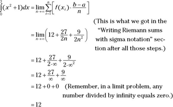
Big surprise.

This result is pretty amazing if you think about it. Using the limit process, you get an exact answer of 12 — sort of like 12.00000000… to an infinite number of decimal places — for the area under the smooth, curving function , based on the areas of flat-topped rectangles that run along the curve in a jagged, sawtooth fashion. Let me guess — the sheer power of this mathematical beauty is bringing tears to your eyes.

Finding the exact area of 12 by using the limit of a Riemann sum is a lot of work (remember, you first had to determine the formula for n right rectangles). This complicated method of integration is comparable to determining a derivative the hard way by using the formal definition that’s based on the difference quotient (see Chapter 9). And just as you stopped using the formal definition of the derivative after you learned the differentiation shortcuts, you won’t have to use the formal definition of the definite integral based on a Riemann sum after you learn the shortcut methods in Chapters 15 and 16 — except, that is, on your final exam.

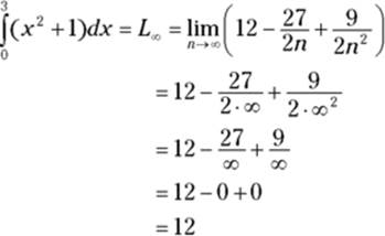
Because the limit of all Riemann sums is the same, the limits at infinity of n left rectangles and n midpoint rectangles — for between x = 0 and x = 3 — should give us the same result as the limit at infinity of nright rectangles. The expressions after the following limit symbols are the formulas for n left rectangles and n midpoint rectangles that appear at the end of the “Writing Riemann sums with sigma notation” section earlier in the chapter. Here’s the left rectangle limit:

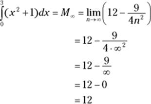
And here’s the midpoint rectangle limit:

If you’re somewhat incredulous that these limits actually give you the exact area under between 0 and 3, you’re not alone. After all, in these limits, as in all limit problems, the arrow-number ( in this example) is only approached; it’s never actually reached. And on top of that, what would it mean to reach infinity? You can’t do it. And regardless of how many rectangles you have, you always have that jagged, sawtooth edge. So how can such a method give you the exact area?

Look at it this way. You can tell from Figures 14-4 and 14-5 that the sum of the areas of left rectangles, regardless of their number, will always be an underestimate (this is the case for functions that are increasing over the span in question). And from Figure 14-6, you can see that the sum of the areas of right rectangles, regardless of how many you have, will always be an overestimate (for increasing functions). So, because the limits at infinity of the underestimate and the overestimate are both equal to 12, that must be the exact area. (A similar argument works for decreasing functions.)

All Riemann sums for a given problem have the same limit. Not only are the limits at infinity of left, right, and midpoint rectangles the same for a given problem, the limit of any Riemann sum also gives you the same answer. You can have a series of rectangles with unequal widths; you can have a mix of left, right, and midpoint rectangles; or you can construct the rectangles so they touch the curve somewhere other than at their left or right upper corners or at the midpoints of their top sides. The only thing that matters is that, in the limit, the width of all the rectangles tends to zero (and from this it follows that the number of rectangles approaches infinity). This brings us to the following totally extreme, down-and-dirty integration mumbo jumbo that takes all these possibilities into account.

The definite integral (real-McCoy definition): The definite integral from to , , is the number to which all Riemann sums tend as the width of all rectangles tends to zero and as the number of rectangles approaches infinity:

where is the width of the ith rectangle and is the x-coordinate of the point where the ith rectangle touches . (That “” simply guarantees that the width of all the rectangles approaches zero and that the number of rectangles approaches infinity.)

Approximating Area with the Trapezoid Rule and Simpson’s Rule

This section covers two more ways to estimate the area under a function. You can use them if for some reason you only want an estimate and not an exact answer — maybe because you’re asked for that on an exam. But these approximation methods and the others we’ve gone over are useful for another reason. There are certain types of functions for which the exact area method doesn’t work. (It’s beyond the scope of this book to explain why this is the case or exactly what these functions are like, so just take my word for it.) So, using an approximation method may be your only choice if you happen to get one of these uncooperative functions.

The trapezoid rule

With the trapezoid rule, instead of approximating area with rectangles, you do it with — can you guess? — trapezoids. See Figure 14-9.

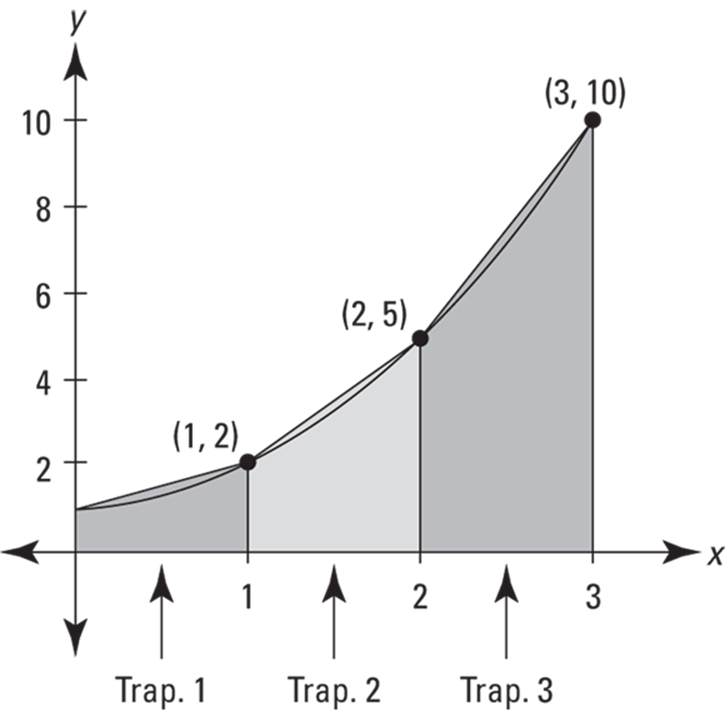
FIGURE 14-9: Three trapezoids approximate the area under between 0 and 3.

Because of the way trapezoids hug the curve, they give you a much better area estimate than either left or right rectangles. And it turns out that a trapezoid approximation is the average of the left rectangle and right rectangle approximations. Can you see why? (Hint: The area of a trapezoid — say trapezoid 2 in Figure 14-9 — is the average of the areas of the two corresponding rectangles in the left and right sums, namely, rectangle number 2 in Figure 14-4 and rectangle 2 in Figure 14-6.)

Table 14-4 lists the trapezoid approximations for the area under between and .

TABLE 14-4 Estimates of the Area Under between and Given by Increasing Numbers of Trapezoids

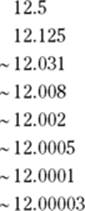
From the look of Figure 14-9, you might expect a trapezoid approximation to be better than a midpoint estimate, but in fact, as a general rule, midpoint estimates are about twice as good as trapezoid estimates. You can confirm this by comparing Tables 14-3 and 14-4. For instance, Table 14-3 lists an area estimate of 11.9990 for 48 midpoint rectangles. This differs from the exact area of 12 by 0.001. The area estimate with 48 trapezoids given in Table 14-4, namely 12.002, differs from 12 by twice as much.

A trapezoid approximation is the average of the corresponding left-rectangle approximation and the right-rectangle approximation. If you’ve already worked out the left- and right-rectangle approximations for a particular function and a certain number of rectangles, you can just average them to get the corresponding trapezoid estimate. If not, here’s the formula:

The trapezoid rule: You can approximate the exact area under a curve between and , , with a sum of trapezoids given by the following formula. In general, the more trapezoids, the better the estimate.

where n is the number of trapezoids, is half the “height” of each sideways trapezoid, and through are the evenly spaced points from to . (By the way, using that half-the-height expression is completely unintuitive considering that the formula for the area of a trapezoid uses its height, not half its height. For extra credit, see if you can figure out why that b - a is divided by 2n instead of just n.)

Even though the formal definition of the definite integral is based on the sum of an infinite number of rectangles, I prefer to think of integration as the limit of the trapezoid rule at infinity. The further you zoom in on a curve, the straighter it gets. When you use a greater and greater number of trapezoids and then zoom in on where the trapezoids touch the curve, the tops of the trapezoids get closer and closer to the curve. If you zoom in “infinitely,” the tops of the “infinitely many” trapezoids become the curve and, thus, the sum of their areas gives you the exact area under the curve. This is a good way to think about why integration produces the exact area — and it makes sense conceptually — but it’s not actually done this way.

Simpson’s rule — that’s Thomas (1710–1761), not Homer (1987–)

Now I really get fancy and draw shapes that are sort of like trapezoids except that instead of having slanting tops, they have curved, parabolic tops. See Figure 14-10.

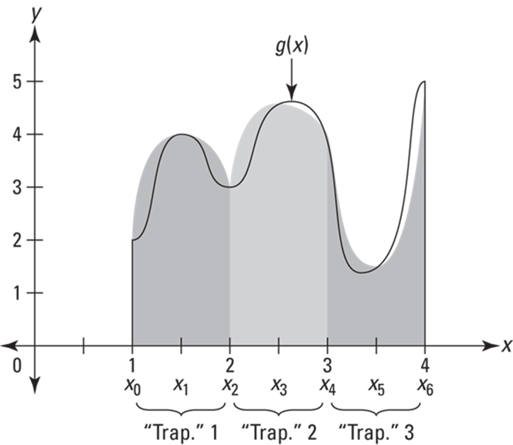
FIGURE 14-10: Three curvy-topped “trapezoids” approximate the area under between 1 and 4.

Note that with Simpson’s rule each “trapezoid” spans two intervals instead of one; in other words, “trapezoid” number 1 goes from to , “trapezoid” 2 goes from to , and so on. Because of this, the total span must always be divided into an even number of intervals.

Simpson’s rule is by far the most accurate approximation method discussed in this chapter. In fact, it gives the exact area for any polynomial function of degree three or less. In general, Simpson’s rule gives a much better estimate than either the midpoint rule or the trapezoid rule.

You can use a midpoint sum with a trapezoid sum to calculate a Simpson sum. A Simpson’s rule sum is sort of an average of a midpoint sum and a trapezoid sum, except that you use the midpoint sum twice in the average. So, if you already have the midpoint sum and the trapezoid sum for some number of rectangles/rapezoids, you can obtain the Simpson’s rule approximation with the following simple average:

Note the subscript of 2n. This means that if you use, say, and , you get a result for  . But , which has six intervals, has only three curvy “trapezoids” because each of them spans two intervals. Thus, the above formula always involves the same number of rectangles, trapezoids, and Simpson’s rule “trapezoids.”

If you don’t have the midpoint and trapezoid sums for the above shortcut, you can use the following formula for Simpson’s rule.

Simpson’s rule: You can approximate the exact area under a curve between and , , with a sum of parabola-topped “trapezoids” given by the following formula. In general, the more “trapezoids,” the better the estimate.

where n is twice the number of “trapezoids” and through are the evenly spaced points from to .

To close this chapter, here’s a warning about functions that go below the x-axis. I didn’t include any such functions in this chapter, because I thought you already had enough to deal with. You see the full explanation and an example in Chapter 17.

Areas below the x-axis count as negative areas. Whether approximating areas with right-, left-, or midpoint rectangles or with the trapezoid rule or Simpson’s rule, or computing exact areas with the definite integral, areas below the x-axis and above the curve count as negative areas.