Discrete Fractional Calculus (2015)
2. Discrete Delta Fractional Calculus and Laplace Transforms
2.5. Composition Rules
Theorem 2.46 (Composition of Fractional Sums).
Assume f is defined on ![]() and μ, ν are positive numbers. Then
and μ, ν are positive numbers. Then
![]()
for ![]()
Proof.
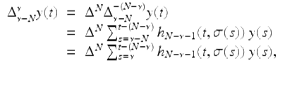
For ![]() , consider
, consider
 =\sum _{ s=a+\nu }^{t-\mu }h_{\mu -1}(t,\sigma (s))\left (\Delta _{a}^{-\nu }f\right )(s) {}\\ & =& \sum _{s=a+\nu }^{t-\mu }h_{\mu -1}(t,\sigma (s))\sum _{r=a}^{s-\nu }h_{\nu -1}(s,\sigma (r))f(r) {}\\ & =& \frac{1} {\Gamma (\mu )\Gamma (\nu )}\sum _{s=a+\nu }^{t-\mu }\sum _{ r=a}^{s-\nu }(t -\sigma (s))^{\underline{\mu -1}}(s -\sigma (r))^{\underline{\nu -1}}f(r) {}\\ & =& \frac{1} {\Gamma (\mu )\Gamma (\nu )}\sum _{r=a}^{t-(\mu +\nu )}\sum _{ s=r+\nu }^{t-\mu }(t -\sigma (s))^{\underline{\mu -1}}(s -\sigma (r))^{\underline{\nu -1}}f(r), {}\\ \end{array}$$](fractional.files/image1258.png)
where in the last step we interchanged the order of summation. Letting ![]() we obtain
we obtain
 {}\\ & =& \frac{1} {\Gamma (\mu )\Gamma (\nu )}\sum _{r=a}^{t-(\mu +\nu )}\left [\sum _{ x=\nu -1}^{t-\mu -r-1}(t - x - r - 2)^{\underline{\mu -1}}x^{\underline{\nu -1}}\right ]f(r) {}\\ & =& \frac{1} {\Gamma (\nu )}\sum _{r=a}^{t-(\mu +\nu )}\left [ \frac{1} {\Gamma (\mu )}\sum _{x=\nu -1}^{(t-r-1)-\mu }(t - r - 1 -\sigma (x))^{\underline{\mu -1}}x^{\underline{\nu -1}}\right ]f(r) {}\\ & =& \frac{1} {\Gamma (\nu )}\sum _{r=a}^{t-(\mu +\nu )}\left [\Delta _{\nu -1}^{-\mu }t^{\underline{\nu -1}}\right ]_{ t\rightarrow t-r-1}f(r). {}\\ \end{array}$$](fractional.files/image1260.png)
But by Theorem 2.38
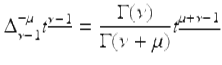
and therefore
& =& \frac{1} {\Gamma (\nu )}\sum _{r=a}^{t-(\mu +\nu )} \frac{\Gamma (\nu )} {\Gamma (\mu +\nu )}(t - r - 1)^{\underline{\mu +\nu -1}}f(r) {}\\ & =& \frac{1} {\Gamma (\mu +\nu )}\sum _{r=a}^{t-(\mu +\nu )}(t -\sigma (r))^{\underline{\mu +\nu -1}}f(r) {}\\ & =& \left (\Delta _{a}^{-(\mu +\nu )}f\right )(t), {}\\ \end{array}$$](fractional.files/image1262.png)
![]() which is one of the desired conclusions. Interchanging μ and ν in the above formula we also get the result
which is one of the desired conclusions. Interchanging μ and ν in the above formula we also get the result
![]()
for ![]() □
□
In the next lemma we give composition rules for an integer difference with a fractional sum and with a fractional difference. Atici and Eloe proved (2.26) with the additional assumption that 0 < k < ν and Holm [123, 125] proved (2.26) in this more general setting.
Lemma 2.47.
Assume ![]() , ν > 0, N − 1 < ν ≤ N. Then
, ν > 0, N − 1 < ν ≤ N. Then
![]()
(2.26)
and
![]()
(2.27)
Proof.
First we prove that
![]()
(2.28)
by induction for ![]() . For the base case we have
. For the base case we have
![$$\displaystyle{\Delta \Delta _{a}^{-1}f(t) = \Delta \bigg[\int _{ a}^{t}f(\tau )\Delta \tau \bigg] = f(t)}$$](fractional.files/image1269.png)
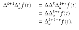
for ![]() Now assume k ≥ 1 and (2.28) holds. Then
Now assume k ≥ 1 and (2.28) holds. Then
![$$\displaystyle\begin{array}{rcl} \Delta ^{k+1}\Delta _{ a}^{k+1}f(t)& & = \Delta ^{k+1}\Delta _{ a+k}^{-1}\Delta _{ a}^{-k}f(t)\qquad \mbox{ using Theorem <InternalRef RefID="FPar4">2.4</InternalRef>6} {}\\ & & = \Delta ^{k}[\Delta \Delta _{ a+k}^{-1}]\Delta _{ a}^{-k}f(t) {}\\ & & = \Delta ^{k}\Delta _{ a}^{-k}f(t)\qquad \mbox{ by the base case with base $a + k$} {}\\ & & = f(t)\qquad \mbox{ by the induction assumption (<InternalRef RefID="Equ88">2.28</InternalRef>)} {}\\ \end{array}$$](fractional.files/image1271.png)
for ![]() Therefore, for k ≥ N
Therefore, for k ≥ N
![]()
and for k < N
![]()
for ![]() Hence for all
Hence for all ![]() we have that (2.26) holds for the case ν = N. It is also true that (2.27) holds when ν = N. Assume for the rest of this proof that N − 1 < ν < N. We will now show by induction that (2.27) holds for
we have that (2.26) holds for the case ν = N. It is also true that (2.27) holds when ν = N. Assume for the rest of this proof that N − 1 < ν < N. We will now show by induction that (2.27) holds for ![]() For the base case k = 1 we have using the Leibniz rule (2.11)
For the base case k = 1 we have using the Leibniz rule (2.11)
![$$\displaystyle\begin{array}{rcl} & & \Delta \Delta _{a}^{\nu }f(t) {}\\ & & = \Delta \bigg[\int _{a}^{t+\nu +1}h_{ -\nu -1}(t,\sigma (\tau ))f(\tau )\Delta \tau \bigg] {}\\ & & =\int _{ a}^{t+\nu +1}h_{ -\nu -2}(t,\sigma (\tau ))f(\tau )\Delta \tau + h_{\nu -1}(\sigma (t),t +\nu +1)f(t +\nu +1) {}\\ & & =\int _{ a}^{t+\nu +1}h_{ -\nu -2}(t,\sigma (\tau ))f(\tau )\Delta \tau + f(t +\nu +1) {}\\ & & =\int _{ a}^{t+\nu +2}h_{ -\nu -2}(t,\sigma (\tau ))f(\tau )\Delta \tau {}\\ & & = \Delta _{a}^{-(-\nu -1)}f(t) {}\\ & & = \Delta _{a}^{1+\nu }f(t). {}\\ \end{array}$$](fractional.files/image1277.png)
Hence the base case
![]()
holds. Now assume k ≥ 1 and
![]()
(2.29)
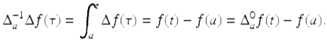
holds. It follows from the induction hypothesis (2.29) and the base case that
Hence (2.27) holds for all ![]() The proof of (2.26) is very similar and is left as an exercise (Exercise 2.23). □
The proof of (2.26) is very similar and is left as an exercise (Exercise 2.23). □
We now prove a composition rule that appears in Holm [125] for a fractional difference with a fractional sum.
Theorem 2.48.
Assume ![]() ν,μ > 0 and N − 1 < ν ≤ N,
ν,μ > 0 and N − 1 < ν ≤ N, ![]() Then
Then
![]()
(2.30)
Proof.
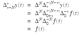
Note that for ![]() ,
,
Hence (2.30) holds. □
Remark 2.49.
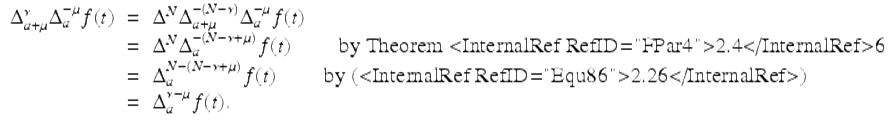
From Theorem 2.46 we saw that we can take fractional sums of fractional sums by adding exponents and by Theorem 2.48 we can take fractional differences of fractional sums by adding exponents. The fundamental theorem of calculus gives us that
Hence we should not expect the fractional sum of a fractional difference can be obtained by adding exponents.
In the next theorem we give a formula for a fractional sum of an integer difference. The first formula in the following Theorem 2.50 is given in Atici et al. [34] and the second formula appears in Holm [125].
Theorem 2.50.
Assume ![]() ,
, ![]() and ν,μ > 0 with N − 1 < μ ≤ N. Then
and ν,μ > 0 with N − 1 < μ ≤ N. Then
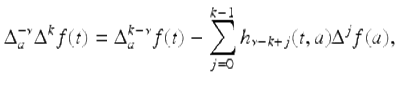
(2.31)
for ![]() , and
, and
(2.32)
for ![]()
Proof.
We first prove that (2.31) holds by induction for ![]() For the base case k = 1 we have using integration by parts and
For the base case k = 1 we have using integration by parts and
![]()
that for ![]()
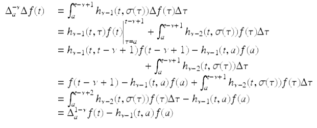
which proves (2.31) for the base case k = 1. Now assume k ≥ 1 and (2.31) holds for that k. Then we have that

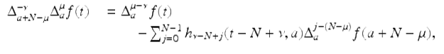
for ![]() Hence (2.31) holds. Next we show that (2.32) holds. To see this suppose now that ν > 0 and μ > 0 with N − 1 < μ ≤ N. Letting
Hence (2.31) holds. Next we show that (2.32) holds. To see this suppose now that ν > 0 and μ > 0 with N − 1 < μ ≤ N. Letting ![]() and
and ![]() (the first point in the domain of g), we have for
(the first point in the domain of g), we have for ![]()
where in this last step, we applied 2.31. □
Finally, we give a composition formula for composing two fractional differences. Note that the rule for this composition is nearly identical to the rule (2.32) for the composition ![]() Theorem 2.51 is given for the specific case
Theorem 2.51 is given for the specific case ![]() by Atici and Eloe in [34].
by Atici and Eloe in [34].
Theorem 2.51.
Let ![]() be given and suppose ν,μ > 0, with N − 1 < ν ≤ N and M − 1 < μ ≤ M. Then for
be given and suppose ν,μ > 0, with N − 1 < ν ≤ N and M − 1 < μ ≤ M. Then for ![]()
(2.33)
for N − 1 < ν < N. If ν = N, then ( 2.33) simplifies to
![]()
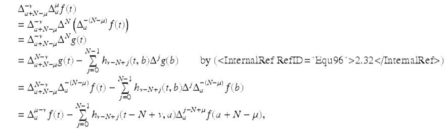
Proof.
Let f, ν, and μ be given as in the statement of the theorem. Lemma 2.47 has already proven the case when ν = N.
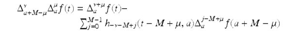
If N − 1 < ν < N, then for ![]() , we have
, we have
![$$\displaystyle\begin{array}{rcl} & & \Delta _{a+M-\mu }^{\nu }\Delta _{ a}^{\mu }f(t) {}\\ & & = \Delta ^{N}\left [\Delta _{ a+M-\mu }^{-(N-\nu )}\Delta _{ a}^{\mu }f(t)\right ]\text{, and now using (<InternalRef RefID="Equ137">2.50</InternalRef>),} {}\\ & & = \Delta ^{N}\Bigg[\Delta _{ a}^{-N+\nu +\mu }f(t) {}\\ & & \quad -\sum \limits _{j=0}^{M-1}\Delta _{ a}^{j-M+\mu }f(a + M-\mu )h_{ N-\nu -M+j}(t - M+\mu,a)\Bigg] {}\\ & & = \Delta _{a}^{\nu +\mu }\Delta ^{N}h_{ N-\nu -M+j}(t - M+\mu )f(t) - {}\\ & &\quad \sum \limits _{j=0}^{M-1}\Delta _{ a}^{j-M+\mu }f(a + M-\mu )\Delta ^{N}h_{ N-\nu -M+j}(t - M+\mu,a)\text{ (Lemma <InternalRef RefID="FPar47">2.47</InternalRef>) } {}\\ & & = \Delta _{a}^{\nu +\mu }f(t) - {}\\ & &\quad \sum \limits _{j=0}^{M-1}\Delta _{ a}^{j-M+\mu }f(a + M-\mu )h_{ -\nu -M+j}(t - M+\mu,a) {}\\ & & = \Delta _{a}^{\nu +\mu }f(t) {}\\ & & \quad -\sum _{j=0}^{M-1}\Delta _{ a}^{j-M+\mu }h_{ -\nu -M+\mu }(t - M+\mu )f(a + M-\mu ). {}\\ \end{array}$$](fractional.files/image1306.png)
□
Theorem 2.52 (Variation of Constants Formula).
Assume N ≥ 1 is an integer and N − 1 < ν ≤ N. If ![]() , then the solution of the IVP
, then the solution of the IVP
![]()
(2.34)
![]()
(2.35)
is given by
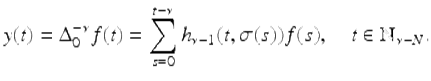
Proof.
Let
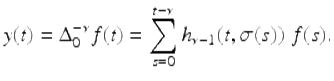
Then by our convention on sums
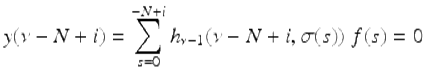
for 0 ≤ i ≤ N − 1, and hence the initial conditions (2.35) are satisfied.
Also, for ![]() ,
,
where in the last step we used the initial conditions (2.35). Hence,
Therefore y is a solution of the fractional difference equation (2.34) on ![]() □
□
Next we use the fractional variation of constants formula to solve a simple fractional IVP.
Example 2.53.
Use the variation of constants formula in Theorem 2.52 to solve the fractional IVP
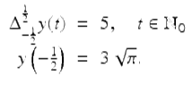
The solution of this IVP is defined on ![]() Note that the corresponding homogeneous fractional difference equation
Note that the corresponding homogeneous fractional difference equation
has the general fractional equation form
![]()
in Theorem 2.43, where
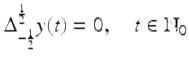
Hence ![]() is a solution of the homogeneous equation
is a solution of the homogeneous equation  and hence (using Theorem 2.52) a general solution of
  is given by
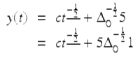
(2.36)
By formula (2.16) we have that
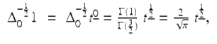
which is the expression that we got for ![]() in Example 2.28. It follows from (2.36) that
in Example 2.28. It follows from (2.36) that
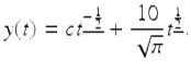
Using the initial condition ![]() we get that c = 3. Therefore, the solution of the given IVP is
we get that c = 3. Therefore, the solution of the given IVP is
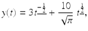
for ![]()
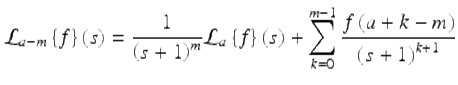
Also, it is often necessary to know how a shifted Laplace transform with respect to its base relates to the original Laplace transform with base a, as is described in the following theorem.
Theorem 2.54.
Let ![]() be given and suppose
be given and suppose ![]() and
and ![]() are of exponential order r > 0. Then for |s + 1| > r,
are of exponential order r > 0. Then for |s + 1| > r,
(2.37)
and
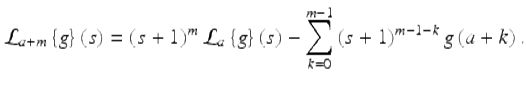
(2.38)
Proof.
Let f, g, r, and m be given as in the statement of this theorem. Then for | s + 1 | > r,
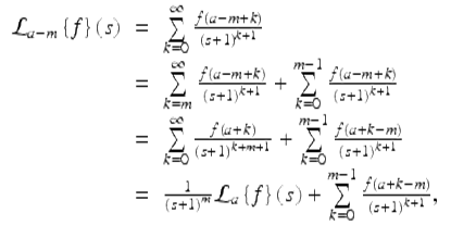
and hence (2.37) holds.
Next, consider
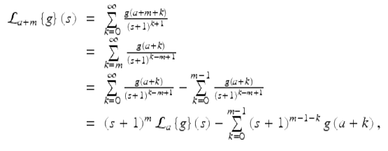
and thus (2.38) holds. □
We leave it as an exercise to verify that applying formulas (2.37) and (2.38) yields
![]()
for | s + 1 | > r.
Recall the definition of the fractional Taylor monomials (Definition 2.24).
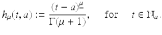
Definition 2.55.
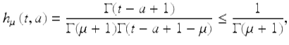
For each ![]() , define the μ-th order Taylor monomial, h μ (t, a), by
, define the μ-th order Taylor monomial, h μ (t, a), by
Theorem 2.56.
If μ ≤ 0 and ![]() , then h μ (t,a) is bounded (and hence is of exponential order r = 1). If μ > 0, then for every r > 1, h μ (t,a) is of exponential order r.
, then h μ (t,a) is bounded (and hence is of exponential order r = 1). If μ > 0, then for every r > 1, h μ (t,a) is of exponential order r.
Proof.
First consider the case that μ ≤ 0 with ![]() . Then for all large
. Then for all large ![]()
implying that h μ is of exponential order one (i.e., bounded).
Next assume that μ > 0, with ![]() chosen so that N − 1 < μ ≤ N. Then for any fixed r > 1,
chosen so that N − 1 < μ ≤ N. Then for any fixed r > 1,
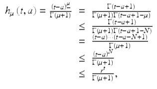
for sufficiently large ![]() .
.
Therefore, h μ (t, a) is of exponential order r for each ![]() and r > 1. It follows from Theorem 2.4 that
and r > 1. It follows from Theorem 2.4 that ![]() exists for | s + 1 | > 1. □
exists for | s + 1 | > 1. □
Remark 2.57.
Note that the fractional Taylor monomials, h μ (t, a) for μ > 0 are examples of functions that are of order r for all r > 1, but are not of order 1 (see Exercise 2.4).
Theorem 2.58.
Let ![]() Then
Then
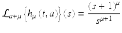
(2.39)
for |s + 1| > 1.
Proof.
For | s + 1 | > 1, consider
![]()
Since ![]() , we have by the binomial theorem that
, we have by the binomial theorem that
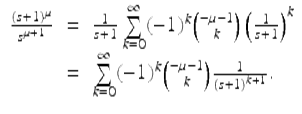
(2.40)
But
![$$\displaystyle\begin{array}{rcl} (-1)^{k}\binom{-\mu - 1}{k}& =& (-1)^{k}\frac{(-\mu - 1)^{\underline{k}}} {k!} \\ & =& (-1)^{k}\frac{(-\mu - 1)(-\mu - 2)\cdots (-\mu - k)} {k!} \\ & =& \frac{(\mu +k)(\mu +k - 1)\cdots (\mu +1)} {k!} \\ & =& \frac{(\mu +k)^{\underline{k}}} {k!} \\ & =& \binom{\mu +k}{k} = \binom{\mu +k}{\mu }\quad \mbox{ by Exercise 1.12, (v)} \\ & =& \frac{(\mu +k)^{\underline{\mu }}} {\Gamma (\mu +1)} \\ & =& \frac{[(a +\mu +k) - a]^{\underline{\mu }}} {\Gamma (\mu +1)} \\ & =& h_{\mu }(a +\mu +k,a). {}\end{array}$$](fractional.files/image1352.png)
(2.41)
Using (2.40) and (2.41), we have that
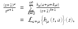
for | s + 1 | > 1. □