Numbers: Their Tales, Types, and Treasures.

Chapter 10: Numbers and Proportions

10.3.EUCLID'S ALGORITHM AND CONTINUED FRACTIONS

In number theory, the method described in figure 10.3 is known as Euclid's algorithm for finding the greatest common divisor of two natural numbers a and b. It allows us to express the proportions between two numbers in the simplest possible way. To illustrate this, we will try to find the greatest common divisor of a = 1,215 and b = 360. We begin by writing

1,215 = 3 × 360 + 135, in general: a = k₁ × b + r₁,
360 = 2 × 135 + 90, b = k₂ × r₁ + r₂,
135 = 1 × 90 + 45, r₁ = k₃ × r₂ + r₃,
90 = 2 × 45 + 0, r₂ = k₄ × r₃ + r₄.

The last nonvanishing remainder is 45. This is the common unit of 1,215 and 360, which is the greatest common divisor. Obviously, 1,215 is 27 × 45 and 360 = 8 × 45, and, therefore,

The algorithm also leads to another nice representation of the quotient of a and b:

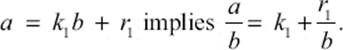
The next step of the algorithm gives b = k₂ × r₁ + r₂. Inserting this in the expression above gives us

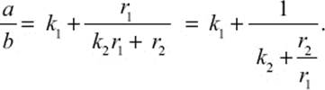
Here, the last expression was obtained by dividing the numerator and denominator by r₁. We continue by inserting r₁ = k₃ × r₂ + r₃, and so on:

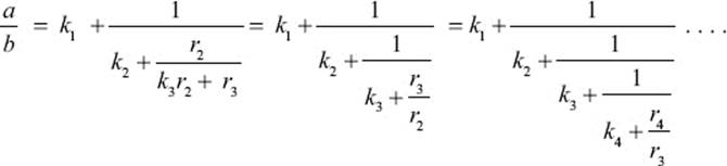
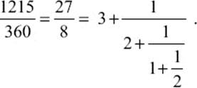
This process can be continued until one of the remainders is zero. In the case of a = 1,215 and b = 360, the remainder r₄ turned out to be 0, while k₁ = 3, k₂ = 2, k₃ = 1, and k₄ = 2. Thus, we obtain the continued-fraction representation

The coefficients in the continued-fraction expansion describe precisely how often the shorter segment fits into the longer segment in each step of the method described in figure 10.3. In that example, the coefficients of the continued fraction expansion are k₁ = 2, k₂ = 1, k₃ = 2, and k₄ = 2. We then get

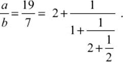
There is another geometric interpretation of this method. Assume that we have a rectangle with length a and width b. Let us try to divide the rectangle into a grid of squares. For example, we start with a rectangle with sides a = 19 and b = 7, as shown in figure 10.4. The coefficients determined from Euclid's algorithm would describe how often the various squares would fit into the rectangle. There are k₁ big squares (with side b), k₂ of the next smaller size, and so on.

Figure 10.4: Tiling of a rectangle.