Process Technology: An Introduction - Haan A.B. 2015

17 Hydrodynamic aspects of scale-up
17.4 Computational fluid dynamics (CFD)

17.4.1 Introduction

Computational fluid dynamics (CFD) is the science of predicting fluid flow, heat transfer, mass transfer, chemical reactions, and related phenomena by solving the mathematical equations which govern these processes, using a numerical algorithm. It is a simulation technique that is used more and more in chemical engineering for design and development, mainly due to the increased capacity in computing power. The simulations allow for an in-depth analysis of the fluid mechanics and local effects in process equipment, which can be used for improved performance, better reliability, more confident scale-up, improved product quality, and higher plant productivity. Today many commercial CFD codes are available, each with different capabilities, special physical models, numerical methods, geometric flexibility, and user interfaces. CFD programs usually consist of three main parts: a presolver, a solver, and a postprocessor (Fig. 17.14). The presolver is used to define the geometry and the properties of the system, the solver performs the actual calculations, and the postprocessor presents the results from the calculations.

17.4.2 Basic principles

The presolver

The first part of the CFD codes is the presolver, where the equipment is defined. If one wants to calculate the extent of mixing in a stirred vessel, for example, several properties have to be provided to the computer-program. First of all, the dimensions of the vessel have to be programmed into the computer, which is often done by a graphical user interface that allows the user to simply draw the vessel or provide the dimensions for the radius and height of the vessel. Next, the shape, size, and position of the stirrer have to be added, as well as the rotation speed. After the geometry is defined, the properties of the liquids, gases, solids, or combination of these have to be provided to the computer. Important data are density as a function of temperature and/or composition, viscosity, heat capacity, and thermal conductivity (if heat-transfer is involved). This data is often provided in the form of simple first-order equations, and possibly by two equations for all properties if a phase-transition is involved. After these properties are defined, initial conditions such as temperature, pressure etc. have to be given.

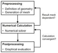
Fig. 17.14: Steps in a CFD simulation.

Grid generation is the next (important) step in programming the problem. To apply CFD, the geometry of interest needs to be divided, or discretized, into a number of computational cells. Discretization is the method of approximating the differential equations by a system of algebraic equations for the variables at some set of discrete locations in space and time. The discrete locations are referred to as the grid or mesh. It is generated because it is virtually impossible to solve all the equations in play for the complete geometry. The number of cells can vary from a few thousand for a simple problem to millions for very large and complicated ones. The size of these squares, the grid, can be chosen to obtain the desired level of detail and to match the difficulty of the problem. Laminar flow, for example, requires a less detailed grid than turbulent flow. In practice, however, the geometry will be a great deal more complicated than a simple square, so the grid will be more complicated as well. Often the grid consists of squares of different sizes and orientations, an example of which is given for a stirred tank in Fig. 17.15. At the height of the stirrer the flow of the liquid is more likely to be turbulent, and therefore a more finely divided grid is used. Further away from the stirrer the fluid flow will be less complicated, and a larger grid can be used.

Once the grid has been created, boundary conditions need to be applied. Pressures, velocities, mass flows, and scalars such as temperature may be specified at inlets; temperature, wall shear rates, or heat fluxes may be set at the walls, and pressure or flow-rate splits may be fixed at outlets. The final step in the presolver, before calculations can begin, is to select the phenomena which have to be considered by the computer. Special attention needs to be paid to accurate modeling of turbulence. The turbulence model chosen should be best suited to the particular flow problem. A wide range of models is available, and understanding the limitations and advantages of the selected one is crucial if the best answer is to be obtained with the minimum computation.

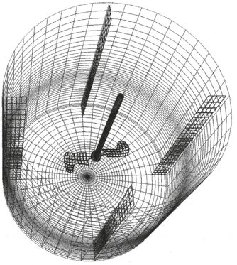
Fig. 17.15: CFD grid structure for an agitated vessel.

The solver

With the grid created, the boundary conditions set, physical properties defined, and models chosen, the calculations can begin. The code will solve the appropriate equations for all grid cells using an iterative procedure. These equations are mainly heat and mass conservation laws, which take the following general form:

(17.6)

In practice, these laws of conservation are often differential equations which are also dependent on each other. Therefore these equations are considered in each single square, and a numerical algorithm is used to solve them. The numerical algorithms can be compared to a mathematically acceptable trial-and-error method, of course with a good theoretical background. Usually the differential equations are formally integrated, and these are solved by an iterative method. Since the geometry can be divided into millions of cells, each with equations containing up to 20 unknowns, it is easy to imagine that a great deal of computer power is needed to solve these systems.

The postprocessor

After solving, an enormous amount of data is obtained, which will be hard to understand in this form. Therefore a postprocessor is always incorporated in CFD codes, usually resulting in colorful pictures or animations of the problem modeled. Different methods are used for visualization of the problem: vector plots, shaded contour plots, or streamlines and/or particle tracking. Temperature and pressure profiles are usually depicted in shaded contour plots, and velocities can be given either as a vector plot, as illustrated in Fig. 17.16 for single-phase flow around the tip of a propeller blade, or as color-coded streamlines.

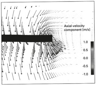
Fig. 17.16: Local formation of vortices at the blade tip.

17.4.3 Applications

Apart from chemical engineering, CFD is extensively used in the automotive industry, airplane design, and racing car development. In all these areas, CFD is used to minimize the air resistance, either to increase top speed or to minimize fuel consumption. To illustrate the successful application to many types of process equipment, a stirred tank reactor and a fluidized bed are discussed.

Stirred tank reactors are one of the most widely used pieces of processing equipment. Traditionally their design is based on parameter correlations such as power draw and impeller pumping capacity. Mixing-time correlations are available, but these are often difficult to extend outside of the experimentally studied parameter range. Stirred tank reactors are a prime example of a hydrodynamically controlled process and have been the focus of extensive CFD modeling in recent years. Fig. 17.17 shows the simulated global flow conditions of a 500 m³ fermenter equipped with three stirrers. These simulations were used to determine the local flow velocity against the cooling coil tubes at the level of the radial-flow impeller.

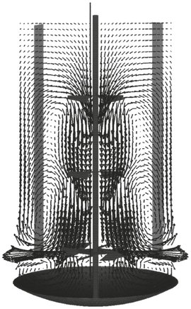
Fig. 17.17: Example of the CFD simulation of a stirred tank fermenter.

Fluidized beds are essentially tanks filled with solid particles, supported by a fine grid below where the gas is introduced. If the amount of gas is high enough, the bed will become fluidized, i.e. the solid particle content will begin to behave like a fluid. CFD is often used in modeling fluidized beds, where complex interactions take place between the solid particles and upward flowing gas. It is used to calculate the formation of gas bubbles, velocities of gas and solids, and the volume fraction of solids, and it is able to indicate whether or not dead zones are present.

Nomenclature