High School Algebra II Unlocked (2016)
Chapter 8. Inferences and Conclusions from Data
Lesson 8.3. Frequency Distributions
REVIEW
Frequencies of data matching individual categories are shown in a bar graph. Frequencies of data that fall within given ranges are shown in a histogram.
One way to analyze data is to look at the relative frequencies of various outcomes, or data points. Let’s compare the data distributions for a simple coin toss and a study of weights of grapes.
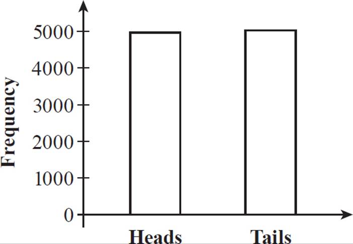
Suppose that an experiment consisting of 10,000 coin tosses has 4980 outcomes of heads and 5020 outcomes of tails. A frequency table for the coin toss experiment would look like this:
|
Outcome |
Frequency |
|
Heads |
4980 |
|
Tails |
5020 |
The frequencies could be shown as a bar graph, allowing you to visually compare the frequency with which each result occurred.
Suppose a researcher weighed 10,000 grapes of a certain variety and categorized the data as number of grapes per each half-gram weight interval, with the results shown in the following frequency table.
Even though we do not know how many employees are in Barbara’s company or what their incomes are, or even the mean of their incomes, we can still determine how a constant added to every element in a population would affect the mean and standard deviation.
Each employee’s income will increase by $5,000 for that year, so the mean of all their incomes will also increase. In a formula for the mean, the sum of all employee incomes will get an added 5000n ($5,000 times n employees in the company), and the total, when divided by n, yields an additional 5000 to what would have been the mean without the bonuses. The mean income will increase by exactly $5,000.
Each of the income data points in the set is increased by the same amount, so the deviation of data points from the mean (which is also increased by the same amount) is not affected. In the formula, each deviation that is squared is the difference (xi − μ). Each xi, or individual employee income, increased by 5000, but the mean, μ, also increased by 5000. The difference ((xi + 5000) − (μ + 5000)) simplifies to (xi − μ), the value of a deviation without a bonus. None of the deviations were affected, so the standard deviation remains the same.
The correct answer is (C).
|
Weight, x (in Grams) |
Frequency (Number of Grapes) |
|
2.0 ≤ x < 2.5 |
10 |
|
2.5 ≤ x < 3.0 |
251 |
|
3.0 ≤ x < 3.5 |
487 |
|
3.5 ≤ x < 4.0 |
552 |
|
4.0 ≤ x < 4.5 |
900 |
|
4.5 ≤ x < 5.0 |
1298 |
|
5.0 ≤ x < 5.5 |
1793 |
|
5.5 ≤ x < 6.0 |
1740 |
|
6.0 ≤ x < 6.5 |
1349 |
|
6.5 ≤ x < 7.0 |
845 |
|
7.0 ≤ x < 7.5 |
520 |
|
7.5 ≤ x < 8.0 |
234 |
|
8.0 ≤ x < 8.5 |
21 |
As with the coin toss results, the information in the frequency table for grape weights can be represented graphically as a frequency distribution. In this case, however, the outcomes are intervals in a continuous range of values, so the frequency distribution graph is a histogram.
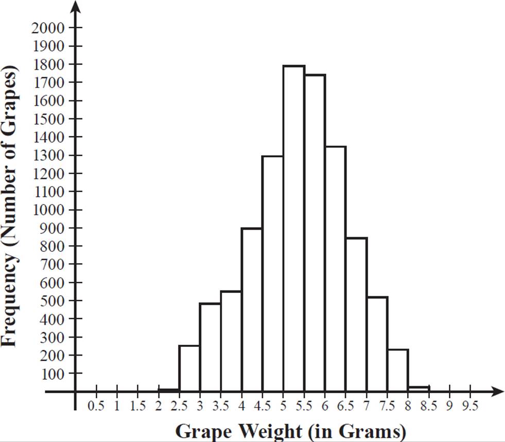
Unlike in the coin toss, where both outcomes occurred with about the same frequency, here it ranges from 10 grapes for an outcome (grape weight) of between 2.0 and 2.5 grams to 1793 grapes for an outcome of between 5.0 and 5.5 grams. Most of the grapes weighed fall within the middle range of weights, centered at about 5.0 to 5.5 grams. Because this is a large data set (and supposing it is representative of the grape variety), we know that if we pick a grape of this variety at random, it is likely to weigh about 5 or 6 grams and very unlikely to weigh 2 grams or 8 grams.
If a sample is large and representative of the target population, then ratios of data in the sample set are likely to be close to the same as ratios of corresponding values in the target population. We can use this proportional reasoning to make inferences about the target population.

Angus surveyed a random sample of 90 students at his school, asking whether they preferred potato chips, tortilla chips, or popcorn. All 90 students responded, with 36 favoring potato chips, 21 favoring tortilla chips, and 33 favoring popcorn. If there are a total of 738 students at Angus’s school, what is a good estimate of the number of students at the school who prefer popcorn to potato chips or tortilla chips?
Out of the 90 students Angus surveyed, 33 students preferred popcorn, so the ratio of popcorn fans to the total number surveyed is 33/90, or 11/30. The sample size is relatively large in relation to the target population size, and it was a randomly chosen sample, so it should be representative of the full student population. So, around the same ratio, 11/30, of the total number of students, 738, should prefer popcorn.
11/30 ⋅ 738 = 270.6
There cannot be a fraction of a person, so we must round off to a whole number, which is appropriate anyway for an estimate. It is likely that about 271 students at Angus’s school prefer popcorn to potato or tortilla chips.

Keep in mind that this is just an estimate, and it’s pretty much equally likely that 270 students at the school prefer popcorn. It’s quite possible that the number is instead 282. There’s even some slight possibility that Angus happened to include the only 33 popcorn fans in the school in his survey, but that is highly unlikely. Rather than just finding a general estimate for a value (such as number of students at a school who prefer popcorn to potato and tortilla chips), it may be more useful to look at the probabilities for various possible values.
If Angus repeated his survey multiple times, each time with another randomly chosen 90-person sample, he could compare results from the surveys, to see how probable it is that 271 is the actual number of students at the school who prefer popcorn, or how close it is to other estimates. The repeated re-sampling method is especially important when trying to draw conclusions about a large target population, such as if Angus wanted to know how many students in all the high schools in the city prefer popcorn.

Here is how you may see proportional reasoning from sample data on the ACT.
Of the 1700 receipts containing large appliance purchases from last month at a certain appliance store, 160 receipts were chosen at random. Each receipt was checked to see which, if any, of the following types of large appliances it included: washer, dryer, refrigerator, or air conditioner. The results were tallied, and the exact percents of receipts that included the large appliances are shown in the diagram below.
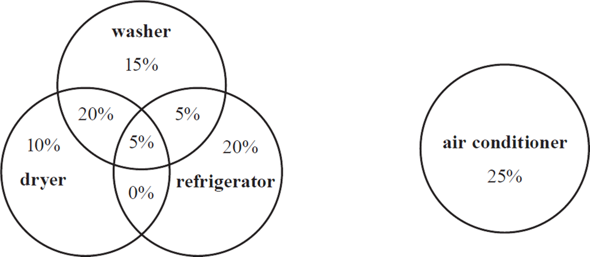
Because this was a random sample, the percents in the sample are estimates for the corresponding percents among all 1700 purchases that included one or more large appliances at the appliance store last month. What estimate does this give for the number of customers who purchased a dryer but none of the other 3 types of large appliances last month?
A. 170
B. 255
C. 340
D. 425
E. 595

Angus recruited some of his friends from other high schools to survey high school students throughout the city as to whether they prefer potato chips, tortilla chips, or popcorn. He instructed each friend to survey multiple randomly-chosen sample groups at his or her high school. Between Angus and his friends, they completed surveys for a total of 100 sample groups of 90 students each, with each sample group randomly selected. The results are shown in the table below, in terms of the frequency (number of sample surveys) with given outcomes (numbers of students who prefer popcorn of the 90 in a given sample survey).
|
Outcome |
Frequency |
|
5 |
1 |
|
19 |
2 |
|
23 |
3 |
|
25 |
5 |
|
27 |
8 |
|
28 |
9 |
|
29 |
8 |
|
30 |
12 |
|
31 |
11 |
|
32 |
10 |
|
33 |
10 |
|
34 |
8 |
|
36 |
5 |
|
38 |
4 |
|
40 |
3 |
|
60 |
1 |
According to this table, what is the probability that a survey of a 90-student sample will have an outcome of exactly 33 students who prefer popcorn? What is the probability of a 90-student sample having an outcome of between 28 and 33 students who prefer popcorn? Which survey results might you question the validity of?
Out of the 100 sample surveys, 10 resulted in an outcome of 33 students preferring popcorn, so the percentage of surveys with this result is 10/100 = 0.1. In other words, there is only a 10% chance that exactly 33 students out of 90 will choose popcorn.
Out of the 100 sample surveys, 9 had an outcome of 28, 8 had an outcome of 29, 12 had an outcome of 30, 11 had an outcome of 31, 10 had an outcome of 32, and 10 had an outcome of 33.
 = 60/100 = 0.6
There is a 60% chance that between 28 and 33 students in a 90-student sample will choose popcorn. So, Angus’s result of 33 students in his initial survey is not unusual. It is within a range of results that occur 60% of the time.
The survey result of only 5 people out of 90 choosing popcorn seems strange, compared to the other results in the table. So does the result of 60 popcorn fans. These may be natural rare occurrences, but they may also be invalid results, perhaps from poorly worded questions in a survey or from a non-random sample, such as the group of students buying snacks at a vending machine that dispenses chips but not popcorn.

Notice that 90% of the sample surveys resulted in outcomes of 25 to 38 students choosing popcorn, per sample. This means a 90% probability that the portion of all high school students in the city who prefer popcorn to potato or tortilla chips is between 25/90 and 38/90.
It is quite a lot of work to coordinate and carry out 100 surveys of 90 people each, with each group chosen through random methods. It also may not be possible to repeatedly re-sample, for various reasons (cost, availability, etc.). In such cases, simulations may allow a researcher to determine the significance of statistical results.

This data presentation is a type of Venn diagram. The percent of customers who purchased only a dryer and no other listed large appliance is shown in the portion of the “dryer” circle that does not overlap with any other circle: 10%. Because 10% of the 160 receipts showed just a dryer purchase, it is likely that 10% of the full population of last month’s large appliance purchasers at the store purchased a dryer and none of the other large appliances.
10% of 1700 = 0.1 ⋅ 1700 = 170
The data provides an estimate of 170 people who purchased a dryer at the appliance store last month, without purchasing an additional washer, refrigerator, or air conditioner. The correct answer is (A).

The student council consists of 3 representatives from each of the 4 grades at the school. To distribute the responsibilities evenly, the principal is supposed to use a random method to choose which student council representative to contact for each question she has. Over the past year, she has contacted individual representatives with questions a total of 320 times. Geoff was contacted 80 times and suspects that the principal is not using random methods, because his number is so high. What are the theoretical probability and the experimental probabilities that the principal will choose Geoff? Create a simulation model of the principal choosing any of the student council representatives with equal probability (the theoretical probability). Use this to simulate 40 outcomes of the principal randomly choosing a representative. What number of outcomes resulted in Geoff being chosen? What would this translate to, proportionally, out of a total of 320 times?
There are 3 student council representatives from each of the 4 grades, so the total number of representatives is 12. If each representative has an equal chance of being chosen, the probability of the principal choosing Geoff is 1/12. This is the theoretical probability.
Over the past year, the principal chose Geoff 80 out of 320 times, so the experimental probability of her choosing Geoff is 80/320, or 1/4. The experimental probability is 3 times the theoretical probability, so the statistic seems meaningful.
One way to simulate the situation is by rolling a fair 12-sided die (a dodecahedron), because the probability of the die landing with any given numbered face up is 1/12, the theoretical probability of the principal choosing any given representative. Let’s assign the number 12 to represent Geoff. Each time the die lands on 12 represents the outcome of the principal contacting Geoff, randomly.
Here are the results of an experiment of rolling a 12-sided die 40 times.

In this simulation, the principal chose Geoff 4 out of 40 times, which represents an experimental probability of 1/10, or 10%. Proportionally, this would translate to randomly choosing Geoff 1/10 ⋅ 320 = 32 times.
We could choose any
number between 1 and
12 to represent Geoff.
We just need to choose
the number in advance
of the simulation,
so that we are not
somehow influenced
by simulation results in
our choice of number.

Notice, however, that this simulation also shows 8 occurrences of the principal randomly choosing representative number 7, which is 1/5 of the 40 simulated results. And, the principal never chose representative number 4 at all in this simulation. As seen here, there is often a great deal of variability in chance processes. The sample size is also not so large. So, although this simulation still suggests that the outcome for Geoff is unusual, it does not clearly prove the unlikeliness of such an outcome.
Another simulation method involves using a random number generator.

Suppose Geoff used a random number generator to generate 320 numbers between 1 and 12, counted the number of times 12 appeared in the set, and repeated this two-step process for a total of 10 data sets (each consisting of 320 numbers). This simulates the principal randomly choosing representatives for 3200 questions (i.e., with each representative equally likely to be chosen). Here is the set of results he got.
{24, 28, 30, 15, 32, 31, 17, 29, 30, 25}
Based on this data, is it statistically meaningful that the principal contacted Geoff with 80 of the questions last year?
None of these results is anywhere near 80, the actual number of times the principal sent Geoff her questions. Even the outcome that is furthest from the expected result is not as different. The expected result is 1/12(320) ≈ 27. The outcome of 15 is furthest from that number in this set, but it is not nearly as far away as 80. Based on this data, the actual outcome of 80 seems statistically significant as a very rare occurrence.
This repeated simulation experiment tells us that a random result of Geoff being chosen 80 times is highly unlikely, so it is probable that the principal was not using truly random sampling methods to choose student council representatives to contact.
