5 Steps to a 5 AP Calculus AB & BC, 2012-2013 Edition (2011)
STEP 4. Review the Knowledge You Need to Score High
Chapter 14. Series (For Calculus BC Students Only)
IN THIS CHAPTER
Summary: In this chapter, you will learn different types of series and the many tests for determining whether they converge or diverge. The types of series include geometric series, p-Series, alternating series, power, and Taylor series. The tests for convergence include the integral test, the comparison test, the limit comparison test, and the ratio test for absolute convergence. These tests involve working with algebraic expressions and lengthy computations. It is important that you carefully work through the practice problems provided in the chapter, and check your solutions with the given explanations.

Key Ideas
![]() Sequences and Series
Sequences and Series
![]() Geometric Series, Harmonic Series, and p-Series
Geometric Series, Harmonic Series, and p-Series
![]() Convergence Tests
Convergence Tests
![]() Alternating Series and Absolute Convergence
Alternating Series and Absolute Convergence
![]() Power Series
Power Series
![]() Taylor Series
Taylor Series
![]() Operations on Series
Operations on Series
![]() Error Bounds
Error Bounds
14.1 Sequences and Series

Main Concepts: Sequences and Series, Convergence
A sequence is a function whose domain is the non-negative integers. It can be expressed as a list of terms {an} = {a1, a2, a3, …, an, …} or by a formula that defines the nth term of the sequence for any value of n. A series ![]() is the sum of the terms of a sequence {an}. Associated with each series is a sequence of partial sums, {sn}, where s1 = a1, s2 = a1 + a2, s3 = a1 + a2 + a3, and in general, sn = a1+ a2 + a3 + … + an.
is the sum of the terms of a sequence {an}. Associated with each series is a sequence of partial sums, {sn}, where s1 = a1, s2 = a1 + a2, s3 = a1 + a2 + a3, and in general, sn = a1+ a2 + a3 + … + an.
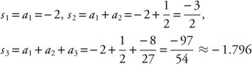
Example 1
Find the first three partial sums of the series  .
.
Step 1: Generate the first three terms of the sequence 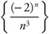 .
.
![]() ,
, ![]() ,
, ![]()
Step 2: Find the partial sums.
Example 2
Find the fifth partial sum of the series  .
.
Step 1: Generate the first five terms of the sequence 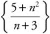 .
.
![]()

![]()
![]()
![]()
Step 2: The fifth partial sum is ![]() .
.
Convergence
The series Σan converges if the sequence of associated partial sums, {sn}, converges. The limit ![]() , where S is a real number, and is the sum of series,
, where S is a real number, and is the sum of series, ![]() . If
. If ![]() and
and ![]() are convergent, then
are convergent, then ![]() and
and ![]() .
.
Example 1
Determine whether the series ![]() converges or diverges. If it converges, find its sum.
converges or diverges. If it converges, find its sum.
Step 1: Find the first few partial sums.
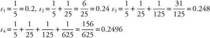
Step 2: The sequence of partial sums {0.2, 0.24, 0.248, 0.2496, …} converges to 0.25, so the series converges, and its sum 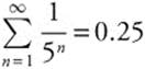 .
.
Example 2
Find the sum of the series ![]() , given that
, given that ![]() and
and ![]() .
.
Step 1: ![]()
Step 2: ![]()
14.2 Types of Series
Main Concepts: p-Series, Harmonic Series, Geometric Series, Decimal Expansion
p-Series
The p-series is a series of the form 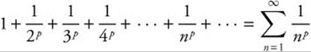 . The p-series converges when p > 1, and diverges when 0 < p ≤ 1.
Harmonic Series
The harmonic series 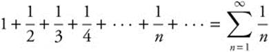 is a p-series with p = 1. The harmonic series diverges.
Geometric Series
A geometric series is a series of the form ![]() where a ≠ 0. A geometric series converges when |r| < 1. The sum of the first n terms of a geometric series is
where a ≠ 0. A geometric series converges when |r| < 1. The sum of the first n terms of a geometric series is ![]() . The sum of the series
. The sum of the series 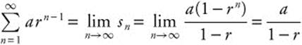 .
.
Example 1
Determine whether the series ![]() converges.
converges. ![]() is a geometric series with a = 1 and
is a geometric series with a = 1 and ![]() . Since r > 1, the series diverges.
. Since r > 1, the series diverges.
Example 2
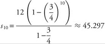
Find the tenth partial sum of the series ![]() .
.
While it is possible to extend the terms of the series and directly compute the tenth partial sum, it is quicker to recognize that this is a geometric series. The ratio of any two subsequent terms is ![]() and the first term is a = 12.
and the first term is a = 12.
Example 3
Find the sum of the series ![]() Since
Since ![]() is a geometric series with a = 12 and
is a geometric series with a = 12 and ![]() ,
, 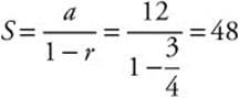 .
.
Decimal Expansion
The rational number equal to the repeating decimal is the sum of the geometric series that represents the repeating decimal.
Example
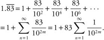
Find the rational number equivalent to ![]() .
.
Step 1: ![]()
Step 2:  is a geometric series with
 ![]() and
and ![]() . The sum of the series is
. The sum of the series is 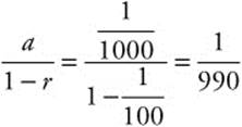 .
.
Step 3:
14.3 Convergence Tests
Main Concepts: Integral Test, Ratio Test, Comparison Test, Limit Comparison Test
Integral Test
If an = f(n) where f is a continuous, positive, decreasing function on [c, ∞), then the series ![]() is convergent if and only if the improper integral
is convergent if and only if the improper integral  exists.
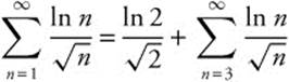
Example 1
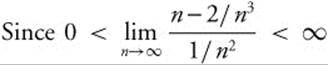
Determine whether the series ![]() converges or diverges.
converges or diverges.
Step 1: ![]() is continuous, positive, and decreasing on the interval [2, ∞).
is continuous, positive, and decreasing on the interval [2, ∞).
Step 2: ![]() . The improper integral exists so
. The improper integral exists so  converges.
Example 2
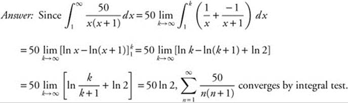
Determine whether the series 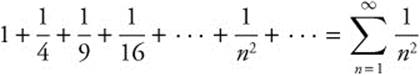 converges or diverges.
Step 1: ![]() is continuous, positive, and decreasing on the interval [1, ∞).
is continuous, positive, and decreasing on the interval [1, ∞).
Step 2: 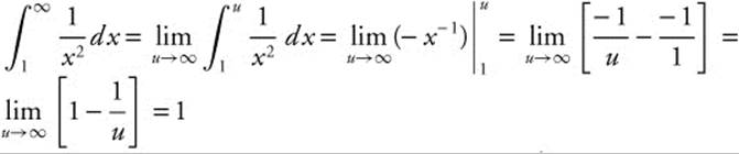
Since the improper integral exists, the series ![]() converges.
converges.
Example 3
Determine whether the series 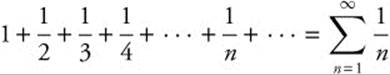 converges or diverges.
Step 1: ![]() is continuous, positive, and decreasing on [1, ∞).
is continuous, positive, and decreasing on [1, ∞).
Step 2: 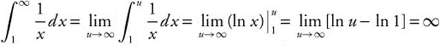 . Since the improper integral does not converge, the series
 ![]() diverges.
diverges.
Example 4
Determine whether the series 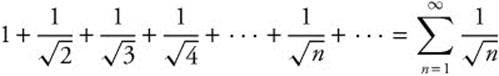 converges or diverges.
Step 1:  is continuous, positive, and decreasing on [1, ∞).
Step 2:  Since the improper integral does not converge, the series
  diverges.
Ratio Test
If ![]() is a series with positive terms and
is a series with positive terms and ![]() , then the series converges. If the limit is greater than 1 or is ∞, the series diverges. If the limit is 1, another test must be used.
, then the series converges. If the limit is greater than 1 or is ∞, the series diverges. If the limit is 1, another test must be used.
Example 1
Determine whether the series  converges or diverges.
Step 1: For all n ≥ 1, ![]() is positive.
is positive.
Step 2:  Since this limit is less than 1, the series converges.
Example 2
Determine whether the series  converges or diverges.
Step 1: For all n ≥ 1,  is positive.
Step 2:  Since this limit is greater than one, the series diverges.
Comparison Test
Suppose ![]() and
and ![]() are series with non-negative terms, and
are series with non-negative terms, and ![]() is known to converge. If a term-by-term comparison shows that for all n, an ≤ bn, then
is known to converge. If a term-by-term comparison shows that for all n, an ≤ bn, then ![]() converges. If
converges. If ![]() diverges, and if for all n, an ≥ bn, then
diverges, and if for all n, an ≥ bn, then ![]() diverges. Common series that may be used for comparison include the geometric series, which converges for r < 1 and diverges for r ≥ 1, and the p-series, which converges for p > 1 and diverges for p ≤ 1.
diverges. Common series that may be used for comparison include the geometric series, which converges for r < 1 and diverges for r ≥ 1, and the p-series, which converges for p > 1 and diverges for p ≤ 1.
Example 1
Determine whether the series ![]() converges or diverges.
converges or diverges.
Step 1: Choose a series for comparison. The series ![]() can be compared to
can be compared to  , the p-series with p = 2. Both series have non-negative terms.
Step 2: A term-by-term comparison shows that ![]() for all values of n.
for all values of n.
Step 3: converges, so ![]() converges.
converges.
Example 2
Determine whether the series ![]() converges or diverges.
converges or diverges.
Step 1: The series  can be compared to
  .
.
Step 2: ![]() , so
, so ![]() for all n ≥ 1.
for all n ≥ 1.
Step 3: ![]() diverges,
diverges, ![]() also diverges.
also diverges.
Limit Comparison Test
If ![]() and
and ![]() are series with positive terms, and if
are series with positive terms, and if ![]() where 0 < L < ∞, then either both series converge or both diverge. By choosing, for one of these, a series that is known to converge, or known to diverge, you can determine whether the other series converges or diverges. Choose a series of a similar form so that the limit expression can be simplified.
where 0 < L < ∞, then either both series converge or both diverge. By choosing, for one of these, a series that is known to converge, or known to diverge, you can determine whether the other series converges or diverges. Choose a series of a similar form so that the limit expression can be simplified.
Example 1
Determine whether the series ![]() converges or diverges. The given series
converges or diverges. The given series 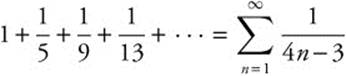 . Choose
  for comparison. Since it has a similar structure, and we know it is a p-series with p = 1, it diverges. The
 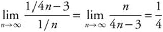 . The limit exists and is greater than zero; therefore, since
  diverges,
 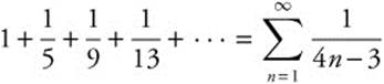 also diverges.
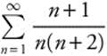
Example 2
Determine whether the series ![]() converges or diverges.
converges or diverges.
Compare to the known convergent ![]() . The
. The 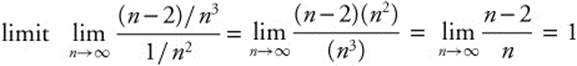 .
.  and
and ![]() converges,
converges, ![]() also converges.
also converges.
14.4 Alternating Series
Main Concepts: Alternating Series, Error Bound, Absolute Convergence
A series whose terms alternate between positive and negative are called alternating series. Alternating series have one of two forms: ![]() or
or ![]() . An alternating series converges if
. An alternating series converges if ![]() and
and ![]() .
.
Example 1
Determine whether the series ![]() converges or diverges.
converges or diverges.
Step 1:
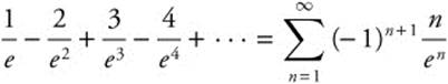
Step 2: Note that ![]() , and in general,
, and in general, ![]() , since multiplying by en+1 gives en > n + 1.
, since multiplying by en+1 gives en > n + 1.
Step 3: 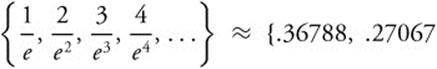 , .14936, .07326, …}, so
 ![]() . Therefore the series converges.
. Therefore the series converges.
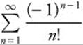
Example 2
Determine whether the series ![]() converges or diverges. If it converges, find its sum.
converges or diverges. If it converges, find its sum.
Step 1: ![]() is a geometric series with a = 4 and
is a geometric series with a = 4 and ![]() . Since r < 1, the series converges.
. Since r < 1, the series converges.
Step 2:
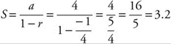
Error Bound
If an alternating series converges to the sum S, then S lies between two consecutive partial sums of the series. If S is approximated by a partial sum sn, the absolute error |S − sn| is less than the next term of the series an + 1, and the sign of S − sn is the same as the coefficient of an+1.
Example
![]() converges to 3.2. This value is greater than sn for n odd, and less than sn for n even. If S is approximated by the third partial sum, s3 = 3.25, the absolute error |S − s3| = |3.2−3.25| = |−0.05| = 0.05, which is clearly less than
converges to 3.2. This value is greater than sn for n odd, and less than sn for n even. If S is approximated by the third partial sum, s3 = 3.25, the absolute error |S − s3| = |3.2−3.25| = |−0.05| = 0.05, which is clearly less than ![]() . The coefficient of a4 is negative, as is S − s3.
. The coefficient of a4 is negative, as is S − s3.
Absolute Convergence
If the series ![]() converges, then
converges, then ![]() converges. A series that converges absolutely converges.
converges. A series that converges absolutely converges.
Example
Determine whether the series 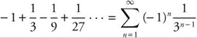 converges.
Step 1: Consider the series 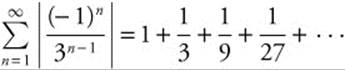 . For this series, s1 = 1,
 ![]() ,
, ![]() ,
, ![]() . The sequence of partial sums,
. The sequence of partial sums, ![]() , converges to 1.5. Or, note that this is a geometric series with a = 1,
, converges to 1.5. Or, note that this is a geometric series with a = 1, ![]() ; thus it converges to
; thus it converges to ![]() .
.
Step 2: 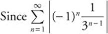 converges,
 ![]() converges.
converges.
14.5 Power Series
Main Concepts: Power Series, Radius and Interval of Convergence
A power series is a series of the form ![]() , where c1, c2, c3, … are constants, and x is a variable.
, where c1, c2, c3, … are constants, and x is a variable.
Radius and Interval of Convergence
A power series centered at x = a converges only for x = a, for all real values of x, or for all x in some open interval (a − R, a + R), called the interval of convergence. The radius of convergence is R. If the series converges on (a − R, a+ R), then it diverges if x < a − R or x > a + R: but convergence or divergence much be investigated individually at x = a − R and at x = a + R.
Example 1
Find the values of x for which the series ![]() converges.
converges.
Step 1: Use the ratio test. 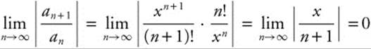
Step 2: The series converges absolutely, so ![]() converges for all real x.
converges for all real x.
Example 2
Find the interval of convergence for the series 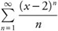 .
.
Step 1: Use the ratio test. 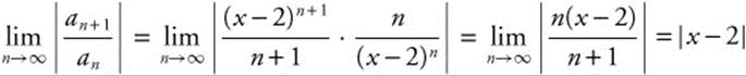
Step 2: The series converges absolutely when |x − 2| < 1, −1 < x − 2 < 1, or 1 < x < 3.
Step 3: When x = 1, the series becomes  . Since 1 >
 ![]() and
and ![]() , this alternating series converges. When x = 3, the series becomes
, this alternating series converges. When x = 3, the series becomes ![]() which is a p-series with p = 1, and therefore diverges. Therefore, the interval of convergence is [1, 3).
which is a p-series with p = 1, and therefore diverges. Therefore, the interval of convergence is [1, 3).
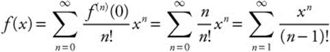
14.6 Taylor Series
Main Concepts: Taylor Series and MacLaurin Series, Common MacLaurin Series
Taylor Series and MacLaurin Series
A Taylor polynomial approximates the value of a function f(x) at the point x = a. If the function and all its derivatives exist at x = a, then on the interval of convergence, the Taylor series  converges to f(x). The MacLaurin series is the name given to a Taylor series centered at x = 0.
Example 1
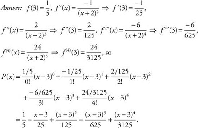
Find the Taylor polynomial of degree 3 for ![]() about the point x = 3.
about the point x = 3.
Step 1: Differentiate: ![]() ,
, ![]() ,
, 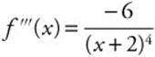 .
.
Step 2: Evaluate: ![]() ,
, ![]() ,
, ![]() ,
, ![]() .
.
Step 3: ![]()
Step 4: 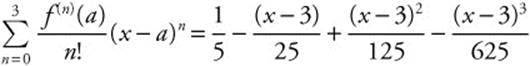
Example 2
A function f(x) is approximated by the third order Taylor series 1 + 2(x − 1) − (x − 1)2 + (x − 1)3 centered at x = 1. Find f′(1) and f′″(1).
Step 1: Compare 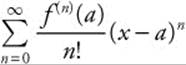 to the given polynomial:
 ![]() ,
, ![]() ,
, ![]() , and
, and ![]() .
.
Step 2: f′(1) = 2 · 1! = 2 and f′″(1) = 1 · 3! = 6.
Example 3
Find the MacLaurin polynomial of degree 4 that approximates f(x) = ln(1 + x).
Step 1: Differentiate: ![]() ,
, ![]() ,
, ![]() ,
, 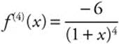 .
.
Step 2: Evaluate: f(0) = 0, f′(0) = 1, f″(0) = −1, f′″(0) = 2, f(4)(0) = −6.
Step 3: ![]()
Example 4
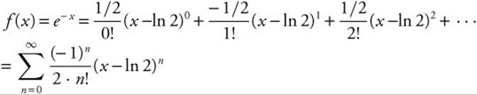
Find the Taylor series for the function f(x) = e−x about the point x = ln 2.
Step 1: f(n)(x) = e−x when n is even and f(n)(x) = − e−x when n is odd.
Step 2: Evaluate ![]() when n is even and
when n is even and ![]() when n is odd.
when n is odd.
Step 3:
Example 5
Find the MacLaurin series for the function f(x) = xex.
Step 1: Investigating the first few derivatives of f(x) = xex shows that f(n)(x) = xex + nex.
Step 2: Evaluating f(n)(x) = xex + nex at x = 0 gives f(n)(0) = n.
Step 3:
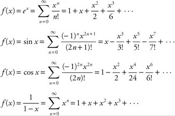
Common MacLaurin Series
MacLaurin Series for the Functions ex, sin x, cos x, and ![]()
Familiarity with these common MacLaurin series will simplify many problems.
14.7 Operations on Series
Main Concepts: Substitution, Differentiation and Integration, Error Bounds
Substitution
New series can be generated by making an appropriate substitution in a known series.
Example 1
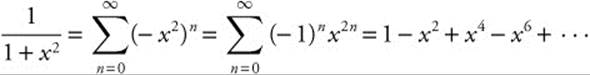
Find the MacLaurin series for ![]() .
.
Step 1: Begin with the known series 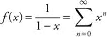 .
.
Step 2: Substitute − x2 for x.
Example 2
Find the first four nonzero terms of the MacLaurin series for f(x) = cos(2x).
Step 1: Begin with the known series ![]()
Step 2: Substitute 2x for x. ![]()
Differentiation and Integration
If a function f(x) is represented by a Taylor series with a non-zero radius of convergence, the derivative f′(x) can be found by differentiating the series term by term. If the series is integrated term-by-term, the resulting series converges to 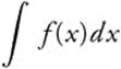 . In either case, the radius of convergence is identical to that of the original series.
Example 1
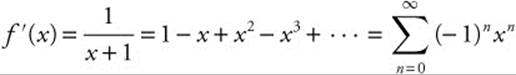
Differentiate the MacLaurin series for f(x) = ln(x + 1) to find the Taylor series expansion for ![]() .
.
Step 1:
![]()
Step 2:
Example 2
Find the MacLaurin series for ![]() .
.
Step 1: We know that 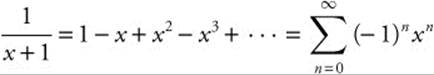 .
.
Step 2: Differentiate: 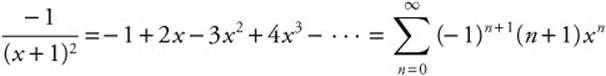 .
.
Step 3: Multiply by − 1.
 .
.
Example 3
Use MacLaurin series to approximate the integral 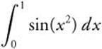 to three decimal place accuracy.
Step 1: Substitute x2 for x in the MacLaurin series representing sin x.

Step 2:
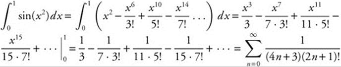
Step 3: For this alternating series, the absolute error for the nth partial sum is less than the n + 1 term so ![]() . We want three decimal place accuracy, so we need
. We want three decimal place accuracy, so we need ![]() or 2000 ≤ (4n + 4)(2n + 2)! This occurs for n ≥ 2.
or 2000 ≤ (4n + 4)(2n + 2)! This occurs for n ≥ 2.
Step 4: Taking the sum ![]() ,
, 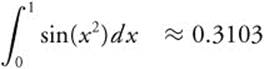 .
.
Error Bounds
The remainder, Rn(x), for a Taylor series is the difference between the actual value of the function f(x) and the nth partial sum that approximates the function. If the function f(x) can be differentiated n + 1 times on an interval containing x0, and if |f(n + 1)(x)| ≤ M for all x in that interval, then ![]() for all x in the interval.
for all x in the interval.
Example 1
Approximate ![]() accurate to three decimal places.
accurate to three decimal places.
Step 1: Substitute ![]() for x in the MacLaurin series representation for ex.
for x in the MacLaurin series representation for ex.
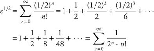
Step 2: For three decimal place accuracy, we want to find the value of n for which the remainder is less than or equal to 0.0005. Choose x0 = 1 in the interval (0, 1). All derivatives of ex are equal to ex, and therefore |f(n + 1)(x)| ≤ e, so M = e. 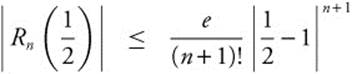 and
and 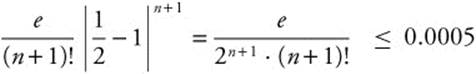 when n ≥ 4.
Step 3: 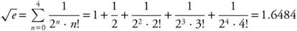
Example 2
Estimate sin 4° accurate to five decimal places.
Step 1: ![]() radians. Substitute
radians. Substitute ![]() for x in the MacLaurin series that represents
for x in the MacLaurin series that represents 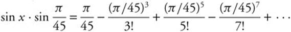
Step 2: For five decimal place accuracy, we must find the value of n for which the absolute error is less than or equal to 5 × 10⁻⁶. For all x, |f(n + 1)(x)| ≤ 1. Choose x0 = 0. 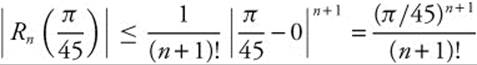 . The absolute error is less than or equal to 5 × 10⁻⁶ for n ≥ 3.
Step 3: 
14.8 Rapid Review
1. Find the sum of the series ![]() .
.
Answer: This is a geometric series with first term 81 and a ratio of ![]() , so
, so 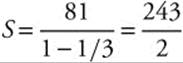 .
.
2. Determine whether the series  converges or diverges.
Answer: 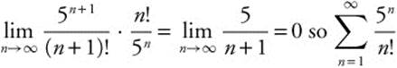 converges by ratio test.
3. Determine whether the series  converges or diverges.
Answer: 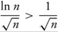 for
for 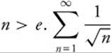 is a p-series with p < 1, so it diverges.
 and
and  diverges by comparison to
  , so the series diverges.
4. Determine whether the series 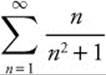 converges or diverges.
Answer: 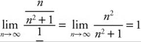 and
and  diverges, so
 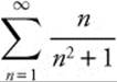 diverges by limit comparison wit .
5. Determine whether the series 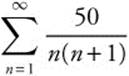 converges or diverges.
6. Find the interval to convergence for the series 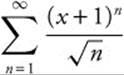 .
.
Answer:  when − 1 < x + 1 < 1 or − 2 ≤ x < 0, the series converges on (−2, 0). When x = −2, the series becomes
 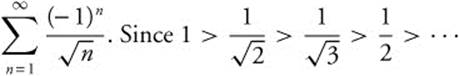 and
and 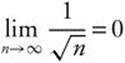 , this alternating series converges. When x = 0, the series becomes
  , which is a p-series with
 ![]() and therefore diverges. Thus, the interval of convergence is [−2, 0).
and therefore diverges. Thus, the interval of convergence is [−2, 0).
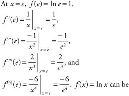
7. Approximate the function ![]() with a fourth degree Taylor polynomial centered at x = 3.
with a fourth degree Taylor polynomial centered at x = 3.
8. Find the MacLaurin series for the function f(x) = e−x and determine its interval of convergence.
Answer: ![]() , substitute − x to find
, substitute − x to find ![]() . The ratio
. The ratio 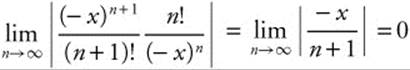 , so the series converges on the interval (− ∞, ∞).
14.9 Practice Problems
Determine whether each series converges or diverges.
1. ![]()
2. ![]()
3. ![]()
4. 
5. 
6. ![]()
7. ![]()
8. ![]()
9. Find the sum of the geometric series 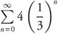 .
.
10. If the sum of the alternating series  is approximated by s50, find the maximum absolute error.
Find the interval of convergence for each series.
11. ![]()
12. ![]()
13. The Taylor series representation of ln x, centered at x = a.
Approximate each function with a fourth degree Taylor polynomial centered at the given value of x.
14. f(x) = ![]() at x = 1.
at x = 1.
15. f(x) = cos πx at ![]() .
.
16. f(x) = ln x at x = e.
Find the MacLaurin series for each function and determine its interval of convergence.
17. ![]()
18. ![]()
19. Estimate sin 9° accurate to three decimal places.
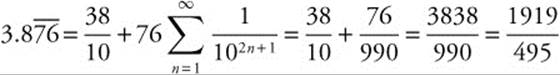
20. Find the rational number equivalent to 1.![]() .
.
14.10 Cumulative Review Problems
21. The movement of an object in the plane is defined by x(t) = ln t, y(t) = t2. Find the speed of the object at the moment when the acceleration is a(t) = ⟨− 1, 2⟩.
22. Find the slope of the tangent line to the curve r = 5 cos 3θ when ![]() .
.
23. 
24. 
25. ![]()
14.11 Solutions to Practice Problems
1.  is a geometric series with an initial term of one and a ratio of
 ![]() . Since the ratio is less than one, the series converges, and
. Since the ratio is less than one, the series converges, and 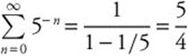 .
.
2. By the ratio test, 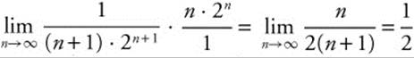 , therefore
  converges.
3. Consider the integral 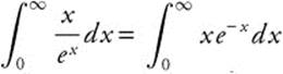 . Integrate by parts, with u = x, du = dx, du = e−x dx, and v = −e−x.
 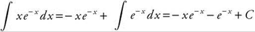 . Therefore,
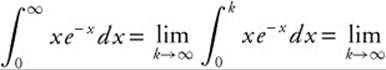
![]() . Since the improper integral converges,
. Since the improper integral converges, ![]() converges.
converges.
4. Use the limit comparison test, comparing to the series ![]() , which is known to diverge. Divide
, which is known to diverge. Divide  . The limit
 ![]() , and
, and ![]() diverges, so the series
diverges, so the series ![]() diverges.
diverges.
5. Use the ratio test, 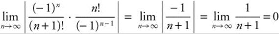 , so the series
 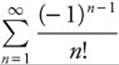 converges absolutely.
6. Use the ratio test. 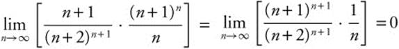 , therefore,
 ![]() converges.
converges.
7.
8. Compare to the p-series with p = 2, ![]() . This series,
. This series,  , is term-by-term less than or equal to the p-series with p = 2. Since that p-series converges,
  converges.
9. The sum of the geometric series 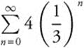 is
is 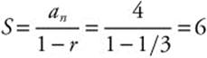 .
.
10. For the alternating series  approximated by s50, the maximum absolute error |Rn| < an + 1, so
 ![]() .
.
11. Examine the ratio of successive terms.  . Since
  , the series will converge when |x| < 1 or − 1 < x < 1. When x = 1, the series becomes
 ![]() . This series is term-by-term smaller than the p-series with p = 2; therefore the series converges. When x = − 1, the series becomes
. This series is term-by-term smaller than the p-series with p = 2; therefore the series converges. When x = − 1, the series becomes  , which also converges. Therefore, the interval of convergence is [− 1, 1 ].
12. The ratio is 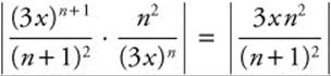 and
and 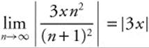 so the series will converge when |3x| < 1. This tells you that − 1 < 3x < 1 and
 ![]() . When
. When ![]() , the series becomes
, the series becomes 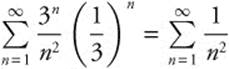 , which is a convergent p-series. When
 ![]() , the series becomes
, the series becomes 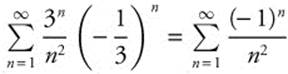 , a convergent alternating series. Therefore the interval of convergence is
  .
.
13. Represent ln x by a Taylor series. Investigate the first few terms by finding and evaluating the derivatives and generating the first few terms.
f(a) = ln a, ![]() ,
, ![]() ,
, ![]() , so ln x can be represented by the
, so ln x can be represented by the 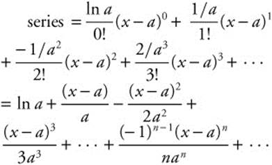 Using the ratio test,
  . The series converges when
 ![]() , that is,
, that is, ![]() . Solving the inequality, you find − a < x − a < a or 0 < x < 2a. When x = 0, the series becomes
. Solving the inequality, you find − a < x − a < a or 0 < x < 2a. When x = 0, the series becomes 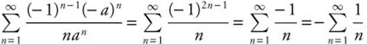 .
.
Since ![]() diverges, this series diverges as well. When x = 2a, the series becomes
diverges, this series diverges as well. When x = 2a, the series becomes 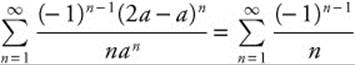 . This alternating series converges; therefore, the interval of convergence is (0, 2a].
14. Calculate the derivatives and evaluate at x = 1. f(x) = ![]() and f(1) = e. f′(x) = 2x
and f(1) = e. f′(x) = 2x![]() and f′(1) = 2e. f″(x) = 4x2
and f′(1) = 2e. f″(x) = 4x2![]() + 2
+ 2![]() and f″(1) = 6e. f‴(x) = 8x3
and f″(1) = 6e. f‴(x) = 8x3 ![]() + 12x
+ 12x![]() and f‴(1) = 20e. f(4)(x) = 16x4
and f‴(1) = 20e. f(4)(x) = 16x4![]() + 48x2
+ 48x2![]() + 12x
+ 12x![]() and f(4)(1) = 76e. Then the function f(x) =
and f(4)(1) = 76e. Then the function f(x) = ![]() can be approximated by
can be approximated by ![]() . Simplifying
. Simplifying ![]() .
.
15.  . Find the derivatives and evaluate at
 ![]() .
. 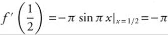 ,
, 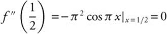 ,
,  , and
, and 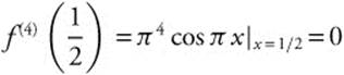 . Then f(x) = cos π x around
 ![]() can be approximated by
can be approximated by 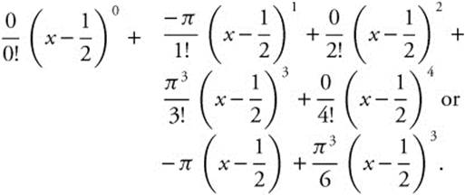 .
.
16.
 .
.
17. Calculate the derivatives and evaluate at 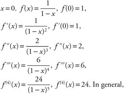 f(n)(0) = n!, so the MacLaurin series
  . The series converges to
 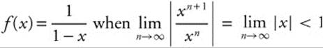 . The series converges on (−1, 1). When x = 1, the series becomes
 ![]() which diverges. When x = − 1, the series becomes
which diverges. When x = − 1, the series becomes ![]() , which diverges. Therefore, the interval of convergence is (−1, 1).
, which diverges. Therefore, the interval of convergence is (−1, 1).
18. Begin with the known series 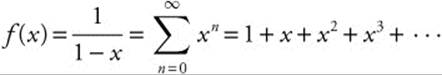 and replace x with − x2. Then
 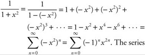 . The series converges to
 ![]() when
when 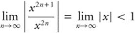 . The series converges on (−1, 1). When x = − 1, the series becomes
  , which diverges. When x = −1, the series becomes
  , which diverges. Therefore, the interval of convergence is (− 1, 1).
19. Use the MacLaurin series 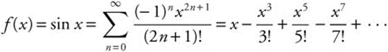 with
with ![]() . Then
. Then 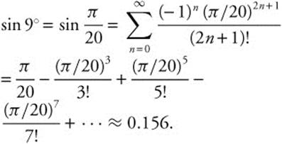 .
.
20.  The geometric series
  converges to
 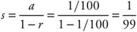 . Therefore,
 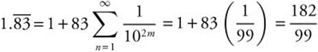 .
.
14.12 Solutions to Cumulative Review Problems
21. ![]() . The acceleration
. The acceleration 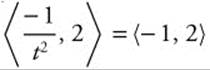 when t = 1. The speed of the object at time t = 1 is
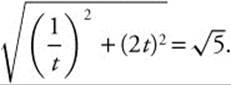
22. x = 5cos 3θ cos θ and y = 5cos 3θ sinθ. ![]() , and
, and ![]() .
. ![]() .
.
Evaluated at ![]() ,
, 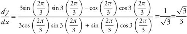 . The slope of the tangent is
 ![]() .
.
23. Integrate by parts, using u = ln x, 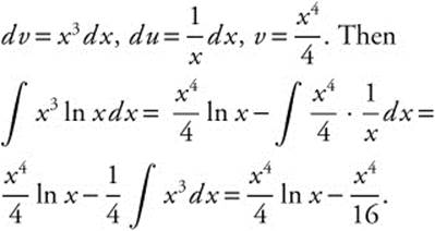 . Consider the limits of integration,
 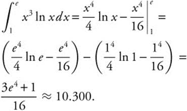 .
.
24. Use partial fraction decomposition. ![]() . Solving the system
. Solving the system 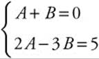 gives A = 1, B = − 1, and
 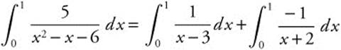 . Then ln
 ![]() − ln
− ln ![]() ln 2 − 2 ln 3 ≈ −0.811.
ln 2 − 2 ln 3 ≈ −0.811.
25. ![]() .
.